In mathematics, the Möbius energy of a knot is a particular knot energy, i.e., a functional on the space of knots. It was discovered by Jun O'Hara, who demonstrated that the energy blows up as the knot's strands get close to one another.[1] This is a useful property because it prevents self-intersection and ensures the result under gradient descent is of the same knot type.
Invariance of Möbius energy under Möbius transformations was demonstrated by Michael Freedman, Zheng-Xu He, and Zhenghan Wang (1994) who used it to show the existence of a  energy minimizer in each isotopy class of a prime knot. They also showed the minimum energy of any knot conformation is achieved by a round circle.[2]
Conjecturally, there is no energy minimizer for composite knots. Robert B. Kusner and John M. Sullivan have done computer experiments with a discretized version of the Möbius energy and concluded that there should be no energy minimizer for the knot sum of two trefoils (although this is not a proof).
Recall that the Möbius transformations of the 3-sphere
 are the ten-dimensional group of angle-preserving diffeomorphisms generated by inversion in 2-spheres. For example, the inversion in the sphere
  is defined by

Consider a rectifiable simple curve  in the Euclidean
3-space
in the Euclidean
3-space  , where
  belongs to
  or
or  . Define its energy by

where  is the shortest arc
distance between
and
is the shortest arc
distance between
and  on the curve. The second term of the
integrand is called a
regularization. It is easy to see that
on the curve. The second term of the
integrand is called a
regularization. It is easy to see that  is
independent of parametrization and is unchanged if
is
independent of parametrization and is unchanged if  is changed by a similarity of . Moreover, the energy of any line is 0, the energy of any circle is
  . In fact, let us use the arc-length parameterization. Denote by
  the length of the curve . Then
![{\displaystyle E(\gamma )=\int _{-\ell /2}^{\ell /2}{}dx\int _{x-\ell /2}^{x+\ell /2}\left[{1 \over |\gamma (x)-\gamma (y)|^{2}}-{1 \over |x-y|^{2}}\right]dy.}](https://wikimedia.org/api/rest_v1/media/math/render/svg/5e43d9199c18fbaa3d6a68120731f9ea2827e48c)
Let  denote a unit circle. We have

and consequently,
![{\displaystyle {\begin{aligned}E(\gamma _{0})&=\int _{-\pi }^{\pi }{}dx\int _{x-\pi }^{x+\pi }\left[{1 \over \left(2\sin {\tfrac {1}{2}}(x-y)\right)^{2}}-{1 \over |x-y|^{2}}\right]dy\\&=4\pi \int _{0}^{\pi }\left[{1 \over \left(2\sin(y/2)\right)^{2}}-{1 \over |y|^{2}}\right]dy\\&=2\pi \int _{0}^{\pi /2}\left[{1 \over \sin ^{2}y}-{1 \over |y|^{2}}\right]dy\\&=2\pi \left[{1 \over u}-\cot u\right]_{u=0}^{\pi /2}=4\end{aligned}}}](https://wikimedia.org/api/rest_v1/media/math/render/svg/a6f5bb41c38af406eadd5473e037bb9b040c7c42)
since  .
.
On the left, the unknot, and a knot equivalent to it. It can be more difficult to determine whether complex knots, such as the one on the right, are equivalent to the unknot.
A knot is created by beginning with a one-dimensional line segment, wrapping it around itself arbitrarily, and then fusing its two free ends together to form a closed loop.[3] Mathematically, we can say a knot  is an injective and continuous function
 ![{\displaystyle K\colon [0,1]\to \mathbb {R} ^{3}}](https://wikimedia.org/api/rest_v1/media/math/render/svg/3527c328346ff511b17bd2fe2ae5f3504df3d2e9) with
with  . Topologists consider knots and other entanglements such as links and braids to be equivalent if the knot can be pushed about smoothly, without intersecting itself, to coincide with another knot. The idea of knot equivalence is to give a precise definition of when two knots should be considered the same even when positioned quite differently in space. A mathematical definition is that two knots
  are equivalent if there is an orientation-preserving homeomorphism
  with
with  , and this is known to be equivalent to existence of ambient isotopy.
The basic problem of knot theory, the recognition problem, is determining the equivalence of two knots. Algorithms exist to solve this problem, with the first given by Wolfgang Haken in the late 1960s. Nonetheless, these algorithms can be extremely time-consuming, and a major issue in the theory is to understand how hard this problem really is. The special case of recognizing the unknot, called the unknotting problem, is of particular interest.[5]
We shall picture a knot by a smooth curve rather than by a polygon. A knot will be represented by a planar diagram. The singularities of the planar diagram will be called crossing points and the regions into which it subdivides the plane regions of the diagram. At each crossing point, two of the four corners will be dotted to indicate which branch through the crossing point is to be thought of as one passing under the other. We number any one region at random, but shall fix the numbers of all remaining regions such that whenever we cross the curve from right to left we must pass from region number  to the region number
  . Clearly, at any crossing point
  , there are two opposite corners of the same number and two opposite corners of the numbers
  and , respectively. The number is referred as the index of . The crossing points are distinguished by two types: the right handed and the left handed, according to which branch through the point passes under or behind the other. At any crossing point of index two dotted corners are of numbers and , respectively, two undotted ones of numbers and . The index of any corner of any region of index is one element of
  . We wish to distinguish one type of knot from another by knot invariants. There is one invariant which is quite simple. It is Alexander polynomial
  with integer coefficient. The Alexander polynomial is symmetric with degree
  :
:  for all knots of
  crossing points. For example, the invariant of an unknotted curve is 1, of an trefoil knot is
  .
.
Let
 denote the standard surface element of
  .
.
We have


For the knot ![{\displaystyle \gamma :[0,1]\rightarrow \mathbb {R} ^{3}}](https://wikimedia.org/api/rest_v1/media/math/render/svg/f571fb855af7f0a45d001b9e9f758d85fe339573) ,
,  ,
,

![{\displaystyle +\int _{t_{1}<t_{2}<t_{3},{\boldsymbol {x}}\in \mathbb {R} ^{3}\setminus \gamma ([0,1])}\omega (\gamma (t_{1})-{\boldsymbol {x}})\wedge \omega (\gamma (t_{2})-{\boldsymbol {x}})\wedge \omega (\gamma (t_{3})-{\boldsymbol {x}})}](https://wikimedia.org/api/rest_v1/media/math/render/svg/6c559a97bed84443bf754509af5182cb9d6b807f)
does not change, if we change the knot in its equivalence class.
Möbius Invariance Property
[edit]Let be a closed curve in  and
and  a Möbius transformation of
  . If
. If  is contained in then
  . If passes through
  then
then  .
.
Theorem A. Among all rectifiable loops  , round circles have the least energy
  and any of least energy parameterizes a round circle.
Proof of Theorem A. Let be a Möbius transformation sending a point of to infinity. The energy  with equality holding if and only if is a straight line. Apply the Möbius invariance property we complete the proof.
Proof of Möbius Invariance Property. It is sufficient to consider how  , an inversion in a sphere, transforms energy. Let be the arc length parameter of a rectifiable closed curve ,
  . Let
. Let
 | | (1) |
and
 | | (2) |
Clearly,  and
and  . It is a short calculation (using the law of cosines) that the first terms transform correctly, i.e.,

Since is arclength for , the regularization term of (1) is the elementary integral
![{\displaystyle \int _{u=0}^{\ell }\left[2\int _{v=\varepsilon }^{\ell /2}{\frac {1}{v^{2}}}\,dv\right]\,du=4-{\frac {2\ell }{\varepsilon }}.}](https://wikimedia.org/api/rest_v1/media/math/render/svg/42db793581695c97a4d59ddb7b30bb809b550904) | | (3) |
Let  be an arclength parameter for
  .
Then
.
Then  where
where  denotes the linear expansion factor of
  . Since is a Lipschitz function and is smooth,
  is Lipschitz, hence, it has weak derivative
  .
.
![{\displaystyle {\begin{aligned}{\rm {{regularization}(2)=}}&\int _{u\in \mathbf {R} /\ell \mathbf {Z} }\left[\int _{|v-u|\geq \varepsilon }{\frac {|(I\circ \gamma )'(v)|\,dv}{D(I\circ \gamma (u),I\circ \gamma (v))^{2}}}\right]|(I\circ \gamma )'(u)|\,du\\=&\int _{\mathbf {R} /\ell \mathbf {Z} }\left[{\frac {4}{L}}-{\frac {1}{\varepsilon _{+}}}-{\frac {1}{\varepsilon _{-}}}\right]\,ds,\end{aligned}}}](https://wikimedia.org/api/rest_v1/media/math/render/svg/6d4250b6416df50fc0c0f611e4713d333ce44218) | | (4) |
where  and
and

and

Since  is uniformly bounded, we have
![{\displaystyle {\begin{aligned}{\frac {1}{\varepsilon _{+}}}=&{\frac {1}{f(u)\varepsilon }}\left[{1+{\varepsilon \over f(u)}\int _{0}^{1}(1-t)f'(u+\varepsilon t)\,dt}\right]^{-1}\\=&{\frac {1}{f(u)\varepsilon }}\left[1-{\frac {\varepsilon }{f(u)}}\int _{0}^{1}(1-t)f'(u+\varepsilon t)\,dt+O(\varepsilon ^{2})\right]\\=&{\frac {1}{f(u)\varepsilon }}-{\frac {1}{f(u)^{2}}}\int _{0}^{1}(1-t)f'(u+\varepsilon t)\,dt+O(\varepsilon ).\end{aligned}}}](https://wikimedia.org/api/rest_v1/media/math/render/svg/0fab1a5cd3107d92025983129dddcf59ea4bdba2)
Similarly,

Then by (4)
![{\displaystyle {\begin{aligned}{\rm {{regularization}\ (2)=}}&4-\int _{0}^{\ell }{\frac {2}{\varepsilon }}\,du+O(\varepsilon )\\&+\int _{u=0}^{\ell }\int _{t=0}^{1}{\frac {(1-t)}{f(u)}}[f'(u+\varepsilon t)-f'(u-\varepsilon t)]\,du\,dt\\=&4-{\frac {2\ell }{\varepsilon }}+O(\varepsilon ).\end{aligned}}}](https://wikimedia.org/api/rest_v1/media/math/render/svg/15f10d9d42ce306698c5c49adc4c5760ae3c6c97) | | (5) |
Comparing (3) and (5), we get
 hence,
  .
.
For the second assertion, let send a point of to infinity. In this case  and, thus, the constant term 4 in (5) disappears.
Freedman–He–Wang conjecture
[edit]The Freedman–He–Wang conjecture (1994) stated that the Möbius energy of nontrivial links in is minimized by the stereographic projection of the standard Hopf link. This was proved in 2012 by Ian Agol, Fernando C. Marques and André Neves, by using Almgren–Pitts min-max theory.[6] Let  ,
,  be a link of 2 components, i.e., a pair of rectifiable closed curves in Euclidean three-space with
  . The Möbius cross energy of the link
  is defined to be

The linking number of is defined by letting


|

|

|

|
|
|
|
|
linking number −2
|
linking number −1
|
linking number 0
|
|
|
|
|
|

|

|
|
|
|
|
|
linking number 1
|
linking number 2
|
linking number 3
|
|
It is not difficult to check that  . If two circles are very far from each other, the cross energy can be made arbitrarily small.
If the linking number
. If two circles are very far from each other, the cross energy can be made arbitrarily small.
If the linking number  is non-zero, the link is called non-split and for the non-split link,
  . So we are interested in the minimal energy of non-split links.
Note that the definition of the energy extends
to any 2-component link in
. So we are interested in the minimal energy of non-split links.
Note that the definition of the energy extends
to any 2-component link in  . The Möbius energy has the remarkable property of being invariant under conformal transformations of . This property is explained as follows. Let
  denote a conformal map. Then
  This condition is called the conformal invariance property of the Möbius cross energy.
Main Theorem. Let , be a non-split link of 2 components link. Then  .
Moreover, if
.
Moreover, if  then there exists a conformal map such that
  and
and  (the standard Hopf link up to orientation and reparameterization).
Given two non-intersecting differentiable curves  , define the Gauss map
  from the torus to the sphere by

The Gauss map of a link in  , denoted by
  , is the Lipschitz map
  defined by
 We denote an open ball in , centered at
  with radius
  , by
, by  . The boundary of this ball is denoted by
  . An intrinsic open ball of
  , centered at
  with radius , is denoted by
  .
We have
.
We have

Thus,

It follows that for almost every  ,
,
 If equality holds at
  , then


If the link is contained in an oriented affine hyperplane with unit normal vector compatible with the orientation, then 
Footnotes


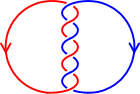
 The left handed trefoil knot.
 The right handed trefoil knot.


