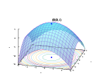
Penalty method
Penalty methods are a certain class of algorithms for solving constrained optimization problems.
A penalty method replaces a constrained optimization problem by a series of unconstrained problems whose solutions ideally converge to the solution of the original constrained problem. The unconstrained problems are formed by adding a term, called a penalty function, to the objective function that consists of a penalty parameter multiplied by a measure of violation of the constraints. The measure of violation is nonzero when the constraints are violated and is zero in the region where constraints are not violated.
Description
[edit]Let us say we are solving the following constrained problem:
subject to
This problem can be solved as a series of unconstrained minimization problems
where
In the above equations, is the exterior penalty function while is the penalty coefficient. When the penalty coefficient is 0, fp=f. In each iteration of the method, we increase the penalty coefficient (e.g. by a factor of 10), solve the unconstrained problem and use the solution as the initial guess for the next iteration. Solutions of the successive unconstrained problems will asymptotically converge to the solution of the original constrained problem.
Common penalty functions in constrained optimization are the quadratic penalty function and the deadzone-linear penalty function[1].
Convergence
[edit]We first consider the set of global optimizers of the original problem, X*.[2]: Thm.9.2.1 Assume that the objective f has bounded level sets, and that the original problem is feasible. Then:
- For every penalty coefficient p, the set of global optimizers of the penalized problem, Xp*, is non-empty.
- For every ε>0, there exists a penalty coefficient p such that the set Xp* is contained in an ε-neighborhood of the set X*.
This theorem is helpful mostly when fp is convex, since in this case, we can find the global optimizers of fp.
A second theorem considers local optimizers.[2]: Thm.9.2.2 Let x* be a non-degenerate local optimizer of the original problem ("nondegenerate" means that the gradients of the active constraints are linearly independent and the second-order sufficient optimality condition is satisfied). Then, there exists a neighborhood V* of x*, and some p0>0, such that for all p>p0, the penalized objective fp has exactly one critical point in V* (denoted by x*(p)), and x*(p) approaches x* as p→∞. Also, the objective value f(x*(p)) is weakly-increasing with p.
Practical applications
[edit]Image compression optimization algorithms can make use of penalty functions for selecting how best to compress zones of colour to single representative values.[3][4] The penalty method is often used in computational mechanics, especially in the Finite element method, to enforce conditions such as e.g. contact.
The advantage of the penalty method is that, once we have a penalized objective with no constraints, we can use any unconstrained optimization method to solve it. The disadvantage is that, as the penalty coefficient p grows, the unconstrained problem becomes ill-conditioned - the coefficients are very large, and this may cause numeric errors and slow convergence of the unconstrained minimization.[2]: Sub.9.2
See also
[edit]Barrier methods constitute an alternative class of algorithms for constrained optimization. These methods also add a penalty-like term to the objective function, but in this case the iterates are forced to remain interior to the feasible domain and the barrier is in place to bias the iterates to remain away from the boundary of the feasible region. They are practically more efficient than penalty methods.
Augmented Lagrangian methods are alternative penalty methods, which allow to get high-accuracy solutions without pushing the penalty coefficient to infinity. This makes the unconstrained penalized problems easier to solve.
Other nonlinear programming algorithms:
- Sequential quadratic programming
- Successive linear programming
- Sequential linear-quadratic programming
- Interior point method
References
[edit]- ^ Boyd, Stephen; Vandenberghe, Lieven (2004). "6.1". Convex Optimization. Cambridge university press. p. 309. ISBN 978-0521833783.
- ^ a b c Nemirovsky and Ben-Tal (2023). "Optimization III: Convex Optimization" (PDF).
- ^ Galar, M.; Jurio, A.; Lopez-Molina, C.; Paternain, D.; Sanz, J.; Bustince, H. (2013). "Aggregation functions to combine RGB color channels in stereo matching". Optics Express. 21 (1): 1247–1257. doi:10.1364/oe.21.001247. hdl:2454/21074. PMID 23389018.
- ^ "Researchers restore image using version containing between 1 and 10 percent of information". Phys.org (Omicron Technology Limited). Retrieved 26 October 2013.
Smith, Alice E.; Coit David W. Penalty functions Handbook of Evolutionary Computation, Section C 5.2. Oxford University Press and Institute of Physics Publishing, 1996.
Coello, A.C.[1]: Theoretical and Numerical Constraint-Handling Techniques Used with Evolutionary Algorithms: A Survey of the State of the Art. Comput. Methods Appl. Mech. Engrg. 191(11-12), 1245-1287
Courant, R. Variational methods for the solution of problems of equilibrium and vibrations. Bull. Amer. Math. Soc., 49, 1–23, 1943.
Wotao, Y. Optimization Algorithms for constrained optimization. Department of Mathematics, UCLA, 2015.


