Seasonality
This article has multiple issues. Please help improve it or discuss these issues on the talk page. (Learn how and when to remove these template messages)
|
In time series data, seasonality refers to the trends that occur at specific regular intervals less than a year, such as weekly, monthly, or quarterly. Seasonality may be caused by various factors, such as weather, vacation, and holidays[1] and consists of periodic, repetitive, and generally regular and predictable patterns in the levels[2] of a time series.
Seasonal fluctuations in a time series can be contrasted with cyclical patterns. The latter occur when the data exhibits rises and falls that are not of a fixed period. Such non-seasonal fluctuations are usually due to economic conditions and are often related to the "business cycle"; their period usually extends beyond a single year, and the fluctuations are usually of at least two years.[3]
Organisations facing seasonal variations, such as ice-cream vendors, are often interested in knowing their performance relative to the normal seasonal variation. Seasonal variations in the labour market can be attributed to the entrance of school leavers into the job market as they aim to contribute to the workforce upon the completion of their schooling. These regular changes are of less interest to those who study employment data than the variations that occur due to the underlying state of the economy; their focus is on how unemployment in the workforce has changed, despite the impact of the regular seasonal variations.[3]
It is necessary for organisations to identify and measure seasonal variations within their market to help them plan for the future. This can prepare them for the temporary increases or decreases in labour requirements and inventory as demand for their product or service fluctuates over certain periods. This may require training, periodic maintenance, and so forth that can be organized in advance. Apart from these considerations, the organisations need to know if variation they have experienced has been more or less than the expected amount, beyond what the usual seasonal variations account for.
Motivation
[edit]There are several main reasons for studying seasonal variation:
- The description of the seasonal effect provides a better understanding of the impact this component has upon a particular series.
- After establishing the seasonal pattern, methods can be implemented to eliminate it from the time-series to study the effect of other components such as cyclical and irregular variations. This elimination of the seasonal effect is referred to as de-seasonalizing or seasonal adjustment of data.
- To use the past patterns of the seasonal variations to contribute to forecasting and the prediction of the future trends, such as in climate normals.
Detection
[edit]The following graphical techniques can be used to detect seasonality:
- A run sequence plot will often show seasonality

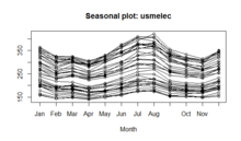
A seasonality plot of US electricity usage - A seasonal plot will show the data from each season overlapped[4]
- A seasonal subseries plot is a specialized technique for showing seasonality
- Multiple box plots can be used as an alternative to the seasonal subseries plot to detect seasonality
- An autocorrelation plot (ACF) and a spectral plot can help identify seasonality.
A really good way to find periodicity, including seasonality, in any regular series of data is to remove any overall trend first and then to inspect time periodicity.[5]
The run sequence plot is a recommended first step for analyzing any time series. Although seasonality can sometimes be indicated by this plot, seasonality is shown more clearly by the seasonal subseries plot or the box plot. The seasonal subseries plot does an excellent job of showing both the seasonal differences (between group patterns) and also the within-group patterns. The box plot shows the seasonal difference (between group patterns) quite well, but it does not show within group patterns. However, for large data sets, the box plot is usually easier to read than the seasonal subseries plot.
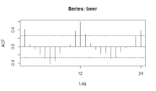
The seasonal plot, seasonal subseries plot, and the box plot all assume that the seasonal periods are known. In most cases, the analyst will in fact, know this. For example, for monthly data, the period is 12 since there are 12 months in a year. However, if the period is not known, the autocorrelation plot can help. If there is significant seasonality, the autocorrelation plot should show spikes at lags equal to the period. For example, for monthly data, if there is a seasonality effect, we would expect to see significant peaks at lag 12, 24, 36, and so on (although the intensity may decrease the further out we go).
An autocorrelation plot (ACF) can be used to identify seasonality, as it calculates the difference (residual amount) between a Y value and a lagged value of Y. The result gives some points where the two values are close together ( no seasonality ), but other points where there is a large discrepancy. These points indicate a level of seasonality in the data.

Semiregular cyclic variations might be dealt with by spectral density estimation.
Calculation
[edit]Seasonal variation is measured in terms of an index, called a seasonal index. It is an average that can be used to compare an actual observation relative to what it would be if there were no seasonal variation. An index value is attached to each period of the time series within a year. This implies that if monthly data are considered there are 12 separate seasonal indices, one for each month. The following methods use seasonal indices to measure seasonal variations of a time-series data.
- Method of simple averages
- Ratio to trend method
- Ratio-to-moving-average method
- Link relatives method
Method of simple averages
[edit]The measurement of seasonal variation by using the ratio-to-moving-average method provides an index to measure the degree of the seasonal variation in a time series. The index is based on a mean of 100, with the degree of seasonality measured by variations away from the base. For example, if we observe the hotel rentals in a winter resort, we find that the winter quarter index is 124. The value 124 indicates that 124 percent of the average quarterly rental occur in winter. If the hotel management records 1436 rentals for the whole of last year, then the average quarterly rental would be 359= (1436/4). As the winter-quarter index is 124, we estimate the number of winter rentals as follows:
359*(124/100)=445;
Here, 359 is the average quarterly rental. 124 is the winter-quarter index. 445 the seasonalized winter-quarter rental.
This method is also called the percentage moving average method. In this method, the original data values in the time-series are expressed as percentages of moving averages. The steps and the tabulations are given below.
Ratio to trend method
[edit]- Find the centered 12 monthly (or 4 quarterly) moving averages of the original data values in the time-series.
- Express each original data value of the time-series as a percentage of the corresponding centered moving average values obtained in step(1). In other words, in a multiplicative time-series model, we get (Original data values) / (Trend values) × 100 = (T × C × S × I) / (T × C) × 100 = (S × I ) × 100.
This implies that the ratio-to-moving average represents the seasonal and irregular components. - Arrange these percentages according to months or quarter of given years. Find the averages over all months or quarters of the given years.
- If the sum of these indices is not 1200 (or 400 for quarterly figures), multiply then by a correction factor = 1200 / (sum of monthly indices). Otherwise, the 12 monthly averages will be considered as seasonal indices.
Ratio-to-moving-average method
[edit]Let us calculate the seasonal index by the ratio-to-moving-average method from the following data:
| Year/Quarters | 1 | 2 | 3 | 4 |
|---|---|---|---|---|
| 1996 | 75 | 60 | 54 | 59 |
| 1997 | 86 | 65 | 63 | 80 |
| 1998 | 90 | 72 | 66 | 85 |
| 1999 | 100 | 78 | 72 | 93 |
Now calculations for 4 quarterly moving averages and ratio-to-moving-averages are shown in the below table.
| Year | Quarter | Original Values(Y) | 4 Figures Moving Total | 4 Figures Moving Average | 2 Figures Moving Total | 2 Figures Moving Average(T) | Ratio-to-Moving-Average(%)(Y)/ (T)*100 |
|---|---|---|---|---|---|---|---|
| 1996 | 1 | 75 | — | — | — | ||
| — | — | ||||||
| 2 | 60 | — | — | — | |||
| 248 | 62.00 | ||||||
| 3 | 54 | 126.75 | 63.375 | 85.21 | |||
| 259 | 64.75 | ||||||
| 4 | 59 | 130.75 | 65.375 | 90.25 | |||
| 264 | 66.00 | ||||||
| 1997 | 1 | 86 | 134.25 | 67.125 | 128.12 | ||
| 273 | 68.25 | ||||||
| 2 | 65 | 141.75 | 70.875 | 91.71 | |||
| 294 | 73.50 | ||||||
| 3 | 63 | 148.00 | 74.00 | 85.13 | |||
| 298 | 74.50 | ||||||
| 4 | 80 | 150.75 | 75.375 | 106.14 | |||
| 305 | 76.25 | ||||||
| 1998 | 1 | 90 | 153.25 | 76.625 | 117.45 | ||
| 308 | 77.00 | ||||||
| 2 | 72 | 155.25 | 77.625 | 92.75 | |||
| 313 | 78.25 | ||||||
| 3 | 66 | 159.00 | 79.50 | 83.02 | |||
| 323 | 80.75 | ||||||
| 4 | 85 | 163.00 | 81.50 | 104.29 | |||
| 329 | 82.25 | ||||||
| 1999 | 1 | 100 | 166.00 | 83.00 | 120.48 | ||
| 335 | 83.75 | ||||||
| 2 | 78 | 169.50 | 84.75 | 92.03 | |||
| 343 | 85.75 | ||||||
| 3 | 72 | — | — | — | |||
| — | — | ||||||
| 4 | 93 | — | — | — | |||
| Years/Quarters | 1 | 2 | 3 | 4 | Total |
|---|---|---|---|---|---|
| 1996 | — | — | 85.21 | 90.25 | |
| 1997 | 128.12 | 91.71 | 85.13 | 106.14 | |
| 1998 | 117.45 | 92.75 | 83.02 | 104.29 | |
| 1999 | 120.48 | 92.04 | — | — | |
| Total | 366.05 | 276.49 | 253.36 | 300.68 | |
| Seasonal Average | 122.01 | 92.16 | 84.45 | 100.23 | 398.85 |
| Adjusted Seasonal Average | 122.36 | 92.43 | 84.69 | 100.52 | 400 |
Now the total of seasonal averages is 398.85. Therefore, the corresponding correction factor would be 400/398.85 = 1.00288. Each seasonal average is multiplied by the correction factor 1.00288 to get the adjusted seasonal indices as shown in the above table.
Link relatives method
[edit]1. In an additive time-series model, the seasonal component is estimated as:
- S = Y – (T + C + I )
where
- S : Seasonal values
- Y : Actual data values of the time-series
- T : Trend values
- C : Cyclical values
- I : Irregular values.
2. In a multiplicative time-series model, the seasonal component is expressed in terms of ratio and percentage as
- Seasonal effect ;
However, in practice the detrending of time-series is done to arrive at .
This is done by dividing both sides of by trend values T so that .
3. The deseasonalized time-series data will have only trend (T ), cyclical (C ) and irregular (I ) components and is expressed as:
- Multiplicative model :
- Additive model: Y – S = (T + S + C + I ) – S = T + C + I
Modeling
[edit]A completely regular cyclic variation in a time series might be dealt with in time series analysis by using a sinusoidal model with one or more sinusoids whose period-lengths may be known or unknown depending on the context. A less completely regular cyclic variation might be dealt with by using a special form of an ARIMA model which can be structured so as to treat cyclic variations semi-explicitly. Such models represent cyclostationary processes.
Another method of modelling periodic seasonality is the use of pairs of Fourier terms. Similar to using the sinusoidal model, Fourier terms added into regression models utilize sine and cosine terms in order to simulate seasonality. However, the seasonality of such a regression would be represented as the sum of sine or cosine terms, instead of a single sine or cosine term in a sinusoidal model. Every periodic function can be approximated with the inclusion of Fourier terms.
The difference between a sinusoidal model and a regression with Fourier terms can be simplified as below:
Sinusoidal Model:
Regression With Fourier Terms:
Seasonal adjustment
[edit]Seasonal adjustment or deseasonalization is any method for removing the seasonal component of a time series. The resulting seasonally adjusted data are used, for example, when analyzing or reporting non-seasonal trends over durations rather longer than the seasonal period. An appropriate method for seasonal adjustment is chosen on the basis of a particular view taken of the decomposition of time series into components designated with names such as "trend", "cyclic", "seasonal" and "irregular", including how these interact with each other. For example, such components might act additively or multiplicatively. Thus, if a seasonal component acts additively, the adjustment method has two stages:
- estimate the seasonal component of variation in the time series, usually in a form that has a zero mean across series;
- subtract the estimated seasonal component from the original time series, leaving the seasonally adjusted series: .[3]
If it is a multiplicative model, the magnitude of the seasonal fluctuations will vary with the level, which is more likely to occur with economic series.[3] When taking seasonality into account, the seasonally adjusted multiplicative decomposition can be written as ; whereby the original time series is divided by the estimated seasonal component.
The multiplicative model can be transformed into an additive model by taking the log of the time series;
SA Multiplicative decomposition:
Taking log of the time series of the multiplicative model: [3]
One particular implementation of seasonal adjustment is provided by X-12-ARIMA.
In regression analysis
[edit]In regression analysis such as ordinary least squares, with a seasonally varying dependent variable being influenced by one or more independent variables, the seasonality can be accounted for and measured by including n-1 dummy variables, one for each of the seasons except for an arbitrarily chosen reference season, where n is the number of seasons (e.g., 4 in the case of meteorological seasons, 12 in the case of months, etc.). Each dummy variable is set to 1 if the data point is drawn from the dummy's specified season and 0 otherwise. Then the predicted value of the dependent variable for the reference season is computed from the rest of the regression, while for any other season it is computed using the rest of the regression and by inserting the value 1 for the dummy variable for that season.
Related patterns
[edit]It is important to distinguish seasonal patterns from related patterns. While a seasonal pattern occurs when a time series is affected by the season or the time of the year, such as annual, semiannual, quarterly, etc. A cyclic pattern, or simply a cycle, occurs when the data exhibit rises and falls in other periods, i.e., much longer (e.g., decadal) or much shorter (e.g., weekly) than seasonal. A quasiperiodicity is a more general, irregular periodicity.
See also
[edit]References
[edit]- ^ "Seasonality". |title=Influencing Factors|
- ^ "Archived copy". Archived from the original on 2015-05-18. Retrieved 2015-05-13.
{{cite web}}: CS1 maint: archived copy as title (link) - ^ a b c d e 6.1 Time series components - OTexts.
- ^ 2.1 Graphics - OTexts.
- ^ "time series - What method can be used to detect seasonality in data?". Cross Validated.
Further reading
[edit]- Franses, Philip Hans (1996). Periodicity and Stochastic Trends in Economic Time Series. New York: Oxford University Press. ISBN 0-19-877454-0.
- Ghysels, Eric; Osborn, Denise R. (2001). The Econometric Analysis of Seasonal Time Series. Cambridge: Cambridge University Press. ISBN 0-521-56588-X.
- Hylleberg, Svend (1986). Seasonality in Regression. Orlando: Academic Press. ISBN 0-12-363455-5.
- Hyndman, Rob J.; Athansopoulos, George (2021). Forecasting: practice and principles (3rd ed.). ISBN 978-0-9875071-3-6.
External links
[edit] Media related to Seasonality at Wikimedia Commons
- Seasonality at NIST/SEMATECH e-Handbook of Statistical Methods
![]() This article incorporates public domain material from NIST/SEMATECH e-Handbook of Statistical Methods. National Institute of Standards and Technology.
This article incorporates public domain material from NIST/SEMATECH e-Handbook of Statistical Methods. National Institute of Standards and Technology.


