Вязкость
| Вязкость | |
|---|---|
 Моделирование жидкостей различной вязкости. Жидкость слева имеет меньшую вязкость, чем жидкость справа. | |
Общие символы | ч , м |
Выводы из другие количества | µ = G · t |
| Измерение | |

| Part of a series on |
| Continuum mechanics |
|---|

Вязкость жидкости сопротивления является мерой ее деформации при заданной скорости. [1] Для жидкостей это соответствует неформальному понятию «густота»: например, сироп имеет более высокую вязкость, чем вода . [2] Вязкость определяется с научной точки зрения как сила, умноженная на время, разделенное на площадь. Таким образом, единицей измерения в системе СИ являются ньютоны-секунды на квадратный метр или паскаль-секунды. [1]
Вязкость количественно определяет силу внутреннего трения между соседними слоями жидкости, находящимися в относительном движении. [1] Например, когда вязкая жидкость проталкивается через трубку, она течет быстрее вблизи центральной линии трубки, чем вблизи ее стенок. [3] Эксперименты показывают, что для поддержания потока необходимо некоторое напряжение (например, разница давлений между двумя концами трубки). Это связано с тем, что для преодоления трения между слоями жидкости, находящимися в относительном движении, требуется сила. Для трубки с постоянной скоростью потока сила компенсирующей силы пропорциональна вязкости жидкости.
In general, viscosity depends on a fluid's state, such as its temperature, pressure, and rate of deformation. However, the dependence on some of these properties is negligible in certain cases. For example, the viscosity of a Newtonian fluid does not vary significantly with the rate of deformation.
Zero viscosity (no resistance to shear stress) is observed only at very low temperatures in superfluids; otherwise, the second law of thermodynamics requires all fluids to have positive viscosity.[4][5] A fluid that has zero viscosity (non-viscous) is called ideal or inviscid.
For non-Newtonian fluid's viscosity, there are pseudoplastic, plastic, and dilatant flows that are time-independent, and there are thixotropic and rheopectic flows that are time-dependent.
Etymology
[edit]The word "viscosity" is derived from the Latin viscum ("mistletoe"). Viscum also referred to a viscous glue derived from mistletoe berries.[6]
Definitions
[edit]Dynamic viscosity
[edit]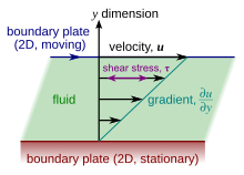

In materials science and engineering, there is often interest in understanding the forces or stresses involved in the deformation of a material. For instance, if the material were a simple spring, the answer would be given by Hooke's law, which says that the force experienced by a spring is proportional to the distance displaced from equilibrium. Stresses which can be attributed to the deformation of a material from some rest state are called elastic stresses. In other materials, stresses are present which can be attributed to the deformation rate over time. These are called viscous stresses. For instance, in a fluid such as water the stresses which arise from shearing the fluid do not depend on the distance the fluid has been sheared; rather, they depend on how quickly the shearing occurs.
Viscosity is the material property which relates the viscous stresses in a material to the rate of change of a deformation (the strain rate). Although it applies to general flows, it is easy to visualize and define in a simple shearing flow, such as a planar Couette flow.
In the Couette flow, a fluid is trapped between two infinitely large plates, one fixed and one in parallel motion at constant speed (see illustration to the right). If the speed of the top plate is low enough (to avoid turbulence), then in steady state the fluid particles move parallel to it, and their speed varies from at the bottom to at the top.[7] Each layer of fluid moves faster than the one just below it, and friction between them gives rise to a force resisting their relative motion. In particular, the fluid applies on the top plate a force in the direction opposite to its motion, and an equal but opposite force on the bottom plate. An external force is therefore required in order to keep the top plate moving at constant speed.


In many fluids, the flow velocity is observed to vary linearly from zero at the bottom to at the top. Moreover, the magnitude of the force, , acting on the top plate is found to be proportional to the speed and the area of each plate, and inversely proportional to their separation :


The proportionality factor is the dynamic viscosity of the fluid, often simply referred to as the viscosity. It is denoted by the Greek letter mu (μ). The dynamic viscosity has the dimensions , therefore resulting in the SI units and the derived units:

![{\displaystyle [\mu ]={\frac {\rm {kg}}{\rm {m{\cdot }s}}}={\frac {\rm {N}}{\rm {m^{2}}}}{\cdot }{\rm {s}}={\rm {Pa{\cdot }s}}=}](https://wikimedia.org/api/rest_v1/media/math/render/svg/a0505c4de127e4d762cc7174f9e205606cbef004)

The aforementioned ratio is called the rate of shear deformation or shear velocity, and is the derivative of the fluid speed in the direction parallel to the normal vector of the plates (see illustrations to the right). If the velocity does not vary linearly with , then the appropriate generalization is:


where , and is the local shear velocity. This expression is referred to as Newton's law of viscosity. In shearing flows with planar symmetry, it is what defines . It is a special case of the general definition of viscosity (see below), which can be expressed in coordinate-free form.


Use of the Greek letter mu () for the dynamic viscosity (sometimes also called the absolute viscosity) is common among mechanical and chemical engineers, as well as mathematicians and physicists.[8][9][10] However, the Greek letter eta () is also used by chemists, physicists, and the IUPAC.[11] The viscosity is sometimes also called the shear viscosity. However, at least one author discourages the use of this terminology, noting that can appear in non-shearing flows in addition to shearing flows.[12]

Kinematic viscosity
[edit]In fluid dynamics, it is sometimes more appropriate to work in terms of kinematic viscosity (sometimes also called the momentum diffusivity), defined as the ratio of the dynamic viscosity (μ) over the density of the fluid (ρ). It is usually denoted by the Greek letter nu (ν):

and has the dimensions , therefore resulting in the SI units and the derived units:

- specific energy multiplied by time energy per unit mass multiplied by time.
![{\displaystyle [\nu ]=\mathrm {\frac {m^{2}}{s}} =\mathrm {{\frac {N{\cdot }m}{kg}}{\cdot }s} =\mathrm {{\frac {J}{kg}}{\cdot }s} =}](https://wikimedia.org/api/rest_v1/media/math/render/svg/abefedddb99ec0896354cfcfcdffd26d00903265)
General definition
[edit]In very general terms, the viscous stresses in a fluid are defined as those resulting from the relative velocity of different fluid particles. As such, the viscous stresses must depend on spatial gradients of the flow velocity. If the velocity gradients are small, then to a first approximation the viscous stresses depend only on the first derivatives of the velocity.[13] (For Newtonian fluids, this is also a linear dependence.) In Cartesian coordinates, the general relationship can then be written as

where is a viscosity tensor that maps the velocity gradient tensor onto the viscous stress tensor .[14] Since the indices in this expression can vary from 1 to 3, there are 81 "viscosity coefficients" in total. However, assuming that the viscosity rank-2 tensor is isotropic reduces these 81 coefficients to three independent parameters , , :


and furthermore, it is assumed that no viscous forces may arise when the fluid is undergoing simple rigid-body rotation, thus , leaving only two independent parameters.[13] The most usual decomposition is in terms of the standard (scalar) viscosity and the bulk viscosity such that and . In vector notation this appears as:


![{\displaystyle {\boldsymbol {\tau }}=\mu \left[\nabla \mathbf {v} +(\nabla \mathbf {v} )^{\mathrm {T} }\right]-\left({\frac {2}{3}}\mu -\kappa \right)(\nabla \cdot \mathbf {v} )\mathbf {\delta } ,}](https://wikimedia.org/api/rest_v1/media/math/render/svg/c881ede5c0e043dbe36b7b5a30b4c6bf92204e5a)
where is the unit tensor.[12][15] This equation can be thought of as a generalized form of Newton's law of viscosity.

The bulk viscosity (also called volume viscosity) expresses a type of internal friction that resists the shearless compression or expansion of a fluid. Knowledge of is frequently not necessary in fluid dynamics problems. For example, an incompressible fluid satisfies and so the term containing drops out. Moreover, is often assumed to be negligible for gases since it is in a monatomic ideal gas.[12] One situation in which can be important is the calculation of energy loss in sound and shock waves, described by Stokes' law of sound attenuation, since these phenomena involve rapid expansions and compressions.

The defining equations for viscosity are not fundamental laws of nature, so their usefulness, as well as methods for measuring or calculating the viscosity, must be established using separate means. A potential issue is that viscosity depends, in principle, on the full microscopic state of the fluid, which encompasses the positions and momenta of every particle in the system.[16] Such highly detailed information is typically not available in realistic systems. However, under certain conditions most of this information can be shown to be negligible. In particular, for Newtonian fluids near equilibrium and far from boundaries (bulk state), the viscosity depends only space- and time-dependent macroscopic fields (such as temperature and density) defining local equilibrium.[16][17]
Nevertheless, viscosity may still carry a non-negligible dependence on several system properties, such as temperature, pressure, and the amplitude and frequency of any external forcing. Therefore, precision measurements of viscosity are only definedwith respect to a specific fluid state.[18] To standardize comparisons among experiments and theoretical models, viscosity data is sometimes extrapolated to ideal limiting cases, such as the zero shear limit, or (for gases) the zero density limit.
Momentum transport
[edit]Transport theory provides an alternative interpretation of viscosity in terms of momentum transport: viscosity is the material property which characterizes momentum transport within a fluid, just as thermal conductivity characterizes heat transport, and (mass) diffusivity characterizes mass transport.[19] This perspective is implicit in Newton's law of viscosity, , because the shear stress has units equivalent to a momentum flux, i.e., momentum per unit time per unit area. Thus, can be interpreted as specifying the flow of momentum in the direction from one fluid layer to the next. Per Newton's law of viscosity, this momentum flow occurs across a velocity gradient, and the magnitude of the corresponding momentum flux is determined by the viscosity.


The analogy with heat and mass transfer can be made explicit. Just as heat flows from high temperature to low temperature and mass flows from high density to low density, momentum flows from high velocity to low velocity. These behaviors are all described by compact expressions, called constitutive relations, whose one-dimensional forms are given here:
![{\displaystyle {\begin{aligned}\mathbf {J} &=-D{\frac {\partial \rho }{\partial x}}&&{\text{(Fick's law of diffusion)}}\\[5pt]\mathbf {q} &=-k_{t}{\frac {\partial T}{\partial x}}&&{\text{(Fourier's law of heat conduction)}}\\[5pt]\tau &=\mu {\frac {\partial u}{\partial y}}&&{\text{(Newton's law of viscosity)}}\end{aligned}}}](https://wikimedia.org/api/rest_v1/media/math/render/svg/6380b89b0d24d9c9deb9ef04f333430b073c45cc)
where is the density, and are the mass and heat fluxes, and and are the mass diffusivity and thermal conductivity.[20] The fact that mass, momentum, and energy (heat) transport are among the most relevant processes in continuum mechanics is not a coincidence: these are among the few physical quantities that are conserved at the microscopic level in interparticle collisions. Thus, rather than being dictated by the fast and complex microscopic interaction timescale, their dynamics occurs on macroscopic timescales, as described by the various equations of transport theory and hydrodynamics.


Newtonian and non-Newtonian fluids
[edit]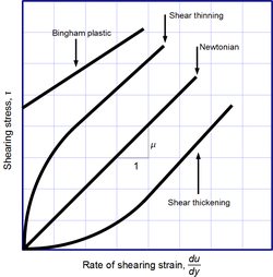
Newton's law of viscosity is not a fundamental law of nature, but rather a constitutive equation (like Hooke's law, Fick's law, and Ohm's law) which serves to define the viscosity . Its form is motivated by experiments which show that for a wide range of fluids, is independent of strain rate. Such fluids are called Newtonian. Gases, water, and many common liquids can be considered Newtonian in ordinary conditions and contexts. However, there are many non-Newtonian fluids that significantly deviate from this behavior. For example:
- Shear-thickening (dilatant) liquids, whose viscosity increases with the rate of shear strain.
- Shear-thinning liquids, whose viscosity decreases with the rate of shear strain.
- Thixotropic liquids, that become less viscous over time when shaken, agitated, or otherwise stressed.
- Rheopectic liquids, that become more viscous over time when shaken, agitated, or otherwise stressed.
- Bingham plastics that behave as a solid at low stresses but flow as a viscous fluid at high stresses.
Trouton's ratio is the ratio of extensional viscosity to shear viscosity. For a Newtonian fluid, the Trouton ratio is 3.[21][22] Shear-thinning liquids are very commonly, but misleadingly, described as thixotropic.[23]
Viscosity may also depend on the fluid's physical state (temperature and pressure) and other, external, factors. For gases and other compressible fluids, it depends on temperature and varies very slowly with pressure. The viscosity of some fluids may depend on other factors. A magnetorheological fluid, for example, becomes thicker when subjected to a magnetic field, possibly to the point of behaving like a solid.
In solids
[edit]The viscous forces that arise during fluid flow are distinct from the elastic forces that occur in a solid in response to shear, compression, or extension stresses. While in the latter the stress is proportional to the amount of shear deformation, in a fluid it is proportional to the rate of deformation over time. For this reason, James Clerk Maxwell used the term fugitive elasticity for fluid viscosity.
However, many liquids (including water) will briefly react like elastic solids when subjected to sudden stress. Conversely, many "solids" (even granite) will flow like liquids, albeit very slowly, even under arbitrarily small stress.[24] Such materials are best described as viscoelastic—that is, possessing both elasticity (reaction to deformation) and viscosity (reaction to rate of deformation).
Viscoelastic solids may exhibit both shear viscosity and bulk viscosity. The extensional viscosity is a linear combination of the shear and bulk viscosities that describes the reaction of a solid elastic material to elongation. It is widely used for characterizing polymers.
In geology, earth materials that exhibit viscous deformation at least three orders of magnitude greater than their elastic deformation are sometimes called rheids.[25]
Measurement
[edit]Viscosity is measured with various types of viscometers and rheometers. Close temperature control of the fluid is essential to obtain accurate measurements, particularly in materials like lubricants, whose viscosity can double with a change of only 5 °C. A rheometer is used for fluids that cannot be defined by a single value of viscosity and therefore require more parameters to be set and measured than is the case for a viscometer.[26]
For some fluids, the viscosity is constant over a wide range of shear rates (Newtonian fluids). The fluids without a constant viscosity (non-Newtonian fluids) cannot be described by a single number. Non-Newtonian fluids exhibit a variety of different correlations between shear stress and shear rate.
One of the most common instruments for measuring kinematic viscosity is the glass capillary viscometer.
In coating industries, viscosity may be measured with a cup in which the efflux time is measured. There are several sorts of cup—such as the Zahn cup and the Ford viscosity cup—with the usage of each type varying mainly according to the industry.
Also used in coatings, a Stormer viscometer employs load-based rotation to determine viscosity. The viscosity is reported in Krebs units (KU), which are unique to Stormer viscometers.
Vibrating viscometers can also be used to measure viscosity. Resonant, or vibrational viscometers work by creating shear waves within the liquid. In this method, the sensor is submerged in the fluid and is made to resonate at a specific frequency. As the surface of the sensor shears through the liquid, energy is lost due to its viscosity. This dissipated energy is then measured and converted into a viscosity reading. A higher viscosity causes a greater loss of energy.[citation needed]
Extensional viscosity can be measured with various rheometers that apply extensional stress.
Volume viscosity can be measured with an acoustic rheometer.
Apparent viscosity is a calculation derived from tests performed on drilling fluid used in oil or gas well development. These calculations and tests help engineers develop and maintain the properties of the drilling fluid to the specifications required.
Nanoviscosity (viscosity sensed by nanoprobes) can be measured by fluorescence correlation spectroscopy.[27]
Units
[edit]The SI unit of dynamic viscosity is the newton-second per square meter (N·s/m2), also frequently expressed in the equivalent forms pascal-second (Pa·s), kilogram per meter per second (kg·m−1·s−1) and poiseuille (Pl). The CGS unit is the poise (P, or g·cm−1·s−1 = 0.1 Pa·s),[28] named after Jean Léonard Marie Poiseuille. It is commonly expressed, particularly in ASTM standards, as centipoise (cP). The centipoise is convenient because the viscosity of water at 20 °C is about 1 cP, and one centipoise is equal to the SI millipascal second (mPa·s).
The SI unit of kinematic viscosity is square meter per second (m2/s), whereas the CGS unit for kinematic viscosity is the stokes (St, or cm2·s−1 = 0.0001 m2·s−1), named after Sir George Gabriel Stokes.[29] In U.S. usage, stoke is sometimes used as the singular form. The submultiple centistokes (cSt) is often used instead, 1 cSt = 1 mm2·s−1 = 10−6 m2·s−1. 1 cSt is 1 cP divided by 1000 kg/m^3, close to the density of water. The kinematic viscosity of water at 20 °C is about 1 cSt.
The most frequently used systems of US customary, or Imperial, units are the British Gravitational (BG) and English Engineering (EE). In the BG system, dynamic viscosity has units of pound-seconds per square foot (lb·s/ft2), and in the EE system it has units of pound-force-seconds per square foot (lbf·s/ft2). The pound and pound-force are equivalent; the two systems differ only in how force and mass are defined. In the BG system the pound is a basic unit from which the unit of mass (the slug) is defined by Newton's Second Law, whereas in the EE system the units of force and mass (the pound-force and pound-mass respectively) are defined independently through the Second Law using the proportionality constant gc.
Kinematic viscosity has units of square feet per second (ft2/s) in both the BG and EE systems.
Nonstandard units include the reyn (lbf·s/in2), a British unit of dynamic viscosity.[30] In the automotive industry the viscosity index is used to describe the change of viscosity with temperature.
The reciprocal of viscosity is fluidity, usually symbolized by or , depending on the convention used, measured in reciprocal poise (P−1, or cm·s·g−1), sometimes called the rhe. Fluidity is seldom used in engineering practice.[citation needed]


At one time the petroleum industry relied on measuring kinematic viscosity by means of the Saybolt viscometer, and expressing kinematic viscosity in units of Saybolt universal seconds (SUS).[31] Other abbreviations such as SSU (Saybolt seconds universal) or SUV (Saybolt universal viscosity) are sometimes used. Kinematic viscosity in centistokes can be converted from SUS according to the arithmetic and the reference table provided in ASTM D 2161.
Molecular origins
[edit]Momentum transport in gases is mediated by discrete molecular collisions, and in liquids by attractive forces that bind molecules close together.[19] Because of this, the dynamic viscosities of liquids are typically much larger than those of gases. In addition, viscosity tends to increase with temperature in gases and decrease with temperature in liquids.
Above the liquid-gas critical point, the liquid and gas phases are replaced by a single supercritical phase. In this regime, the mechanisms of momentum transport interpolate between liquid-like and gas-like behavior.For example, along a supercritical isobar (constant-pressure surface), the kinematic viscosity decreases at low temperature and increases at high temperature, with a minimum in between.[32][33] A rough estimate for the valueat the minimum is

where is the Planck constant, is the electron mass, and is the molecular mass.[33]


In general, however, the viscosity of a system depends in detail on how the molecules constituting the system interact, and there are no simple but correct formulas for it. The simplest exact expressions are the Green–Kubo relations for the linear shear viscosity or the transient time correlation function expressions derived by Evans and Morriss in 1988.[34] Although these expressions are each exact, calculating the viscosity of a dense fluid using these relations currently requires the use of molecular dynamics computer simulations. Somewhat more progress can be made for a dilute gas, as elementary assumptions about how gas molecules move and interact lead to a basic understanding of the molecular origins of viscosity. More sophisticated treatments can be constructed by systematically coarse-graining the equations of motion of the gas molecules. An example of such a treatment is Chapman–Enskog theory, which derives expressions for the viscosity of a dilute gas from the Boltzmann equation.[17]
Pure gases
[edit]Elementary calculation of viscosity for a dilute gas


Viscosity in gases arises principally from the molecular diffusion that transports momentum between layers of flow. An elementary calculation for a dilute gas at temperature and density gives


where is the Boltzmann constant, the molecular mass, and a numerical constant on the order of . The quantity , the mean free path, measures the average distance a molecule travels between collisions. Even without a priori knowledge of , this expression has nontrivial implications. In particular, since is typically inversely proportional to density and increases with temperature, itself should increase with temperature and be independent of density at fixed temperature. In fact, both of these predictions persist in more sophisticated treatments, and accurately describe experimental observations. By contrast, liquid viscosity typically decreases with temperature.[19][35]

For rigid elastic spheres of diameter , can be computed, giving


In this case is independent of temperature, so . For more complicated molecular models, however, depends on temperature in a non-trivial way, and simple kinetic arguments as used here are inadequate. More fundamentally, the notion of a mean free path becomes imprecise for particles that interact over a finite range, which limits the usefulness of the concept for describing real-world gases.[36]

Chapman–Enskog theory
[edit]A technique developed by Sydney Chapman and David Enskog in the early 1900s allows a more refined calculation of .[17] It is based on the Boltzmann equation, which provides a statistical description of a dilute gas in terms of intermolecular interactions.[37] The technique allows accurate calculation of for molecular models that are more realistic than rigid elastic spheres, such as those incorporating intermolecular attractions. Doing so is necessary to reproduce the correct temperature dependence of , which experiments show increases more rapidly than the trend predicted for rigid elastic spheres.[19] Indeed, the Chapman–Enskog analysis shows that the predicted temperature dependence can be tuned by varying the parameters in various molecular models. A simple example is the Sutherland model,[a] which describes rigid elastic spheres with weak mutual attraction. In such a case, the attractive force can be treated perturbatively, which leads to a simple expression for :


where is independent of temperature, being determined only by the parameters of the intermolecular attraction. To connect with experiment, it is convenient to rewrite as


where is the viscosity at temperature . This expression is usually named Sutherland's formula.[38] If is known from experiments at and at least one other temperature, then can be calculated. Expressions for obtained in this way are qualitatively accurate for a number of simple gases. Slightly more sophisticated models, such as the Lennard-Jones potential, or the more flexible Mie potential, may provide better agreement with experiments, but only at the cost of a more opaque dependence on temperature. A further advantage of these more complex interaction potentials is that they can be used to develop accurate models for a wide variety of properties using the same potential parameters. In situations where little experimental data is available, this makes it possible to obtain model parameters from fitting to properties such as pure-fluid vapour-liquid equilibria, before using the parameters thus obtained to predict the viscosities of interest with reasonable accuracy.


In some systems, the assumption of spherical symmetry must be abandoned, as is the case for vapors with highly polar molecules like H2O. In these cases, the Chapman–Enskog analysis is significantly more complicated.[39][40]
Bulk viscosity
[edit]In the kinetic-molecular picture, a non-zero bulk viscosity arises in gases whenever there are non-negligible relaxational timescales governing the exchange of energy between the translational energy of molecules and their internal energy, e.g. rotational and vibrational. As such, the bulk viscosity is for a monatomic ideal gas, in which the internal energy of molecules is negligible, but is nonzero for a gas like carbon dioxide, whose molecules possess both rotational and vibrational energy.[41][42]
Pure liquids
[edit]In contrast with gases, there is no simple yet accurate picture for the molecular origins of viscosity in liquids.
At the simplest level of description, the relative motion of adjacent layers in a liquid is opposed primarily by attractive molecular forcesacting across the layer boundary. In this picture, one (correctly) expects viscosity to decrease with increasing temperature. This is becauseincreasing temperature increases the random thermal motion of the molecules, which makes it easier for them to overcome their attractive interactions.[43]
Опираясь на эту визуализацию, можно построить простую теорию по аналогии с дискретной структурой твердого тела: группы молекул в жидкости. визуализируются как образующие «клетки», окружающие и заключающие в себе отдельные молекулы. [44] These cages can be occupied or unoccupied, andstronger molecular attraction corresponds to stronger cages.Due to random thermal motion, a molecule "hops" between cages at a rate which varies inversely with the strength of molecular attractions. In equilibrium these "hops" are not biased in any direction.On the other hand, in order for two adjacent layers to move relative to each other, the "hops" must be biased in the directionof the relative motion. The force required to sustain this directed motion can be estimated for a given shear rate, leading to
| ( 1 ) |

где – постоянная Авогадро , — постоянная Планка , - объем моля жидкости , а это нормальная температура кипения . Этот результат имеет тот же вид, что и известное эмпирическое соотношение


| ( 2 ) |

где и константы, соответствующие данным. [44] [45] С другой стороны, некоторые авторы выражают осторожность в отношении этой модели. ) могут возникнуть ошибки до 30% При использовании уравнения ( 1 по сравнению с уравнением подгонки ( 2 ) к экспериментальным данным. [44] физические предположения, лежащие в основе уравнения ( 1 ). В более фундаментальном плане подверглись критике [46] Также утверждалось, что экспоненциальная зависимость в уравнении ( 1 ) не обязательно описывает экспериментальные наблюдения более точно, чем более простые неэкспоненциальные выражения. [47] [48]

В свете этих недостатков разработка менее специальной модели представляет практический интерес. Отказ от простоты в пользу точности позволяет написать строгие выражения для вязкости, исходя из фундаментальных уравнений движения молекул. Классическим примером такого подхода является теория Ирвинга–Кирквуда. [49] С другой стороны, такие выражения задаются как средние по многочастичным корреляционным функциям и поэтому их трудно применять на практике.
В целом, выражения, полученные эмпирическим путем (на основе существующих измерений вязкости), кажутся единственным надежным средством расчета вязкости жидкостей. [50]
Изменения локальной атомной структуры наблюдаются в переохлажденных жидкостях при охлаждении ниже равновесной температуры плавления либо через функцию радиального распределения g ( r ) [51] или структурный фактор S ( Q ) [52] Установлено, что они непосредственно ответственны за хрупкость жидкости: отклонение температурной зависимости вязкости переохлажденной жидкости от уравнения Аррениуса (2) за счет модификации энергии активации вязкого течения. В то же время равновесные жидкости подчиняются уравнению Аррениуса.
Смеси и смеси
[ редактировать ]Газовые смеси
[ редактировать ]Ту же молекулярно-кинетическую картину однокомпонентного газа можно применить и к газовой смеси. Например, в подходе Чепмена–Энскога вязкость бинарной смеси газов можно записать через вязкости отдельных компонентов , их соответствующие объемные доли и межмолекулярные взаимодействия. [17]


Что касается однокомпонентного газа, то зависимость На параметры межмолекулярных взаимодействий входит через различные интегралы столкновений, которые не могут быть выражены в замкнутой форме . Чтобы получить полезные выражения для которые разумно соответствуют экспериментальным данным, интегралы столкновений могут быть рассчитаны численно или на основе корреляций. [53] В некоторых случаях интегралы столкновений рассматриваются как подгоночные параметры и подгоняются непосредственно к экспериментальным данным. [54] Это распространенный подход при разработке справочных уравнений вязкости газовой фазы. Примером такой процедуры является подход Сазерленда для однокомпонентного газа, обсуждавшийся выше.
Было показано , что для газовых смесей, состоящих из простых молекул, пересмотренная теория Энскога точно отражает зависимость вязкости как от плотности, так и от температуры в широком диапазоне условий. [55] [53]
Смеси жидкостей
[ редактировать ]Что касается чистых жидкостей, вязкость смеси жидкостей трудно предсказать с помощью молекулярных принципов. Один из методов — расширить представленную выше теорию молекулярной «клетки» на случай чистой жидкости. Это можно сделать с разной степенью сложности. Одним из выражений, полученных в результате такого анализа, является уравнение Ледерера – Регирса для бинарной смеси:

где является эмпирическим параметром, и и – соответствующие мольные доли и вязкости составляющих жидкостей. [56]

Поскольку смешивание является важным процессом в смазочной и нефтяной промышленности, существует множество эмпирических и частных уравнений для прогнозирования вязкости смеси. [56]
Растворы и суспензии
[ редактировать ]Водные растворы
[ редактировать ]В зависимости от растворенного вещества и диапазона концентраций водный раствор электролита может иметь большую или меньшую вязкость по сравнению с чистой водой при той же температуре и давлении. Например, 20%-ный солевой раствор ( хлорид натрия ) имеет вязкость более чем в 1,5 раза больше, чем чистая вода, тогда как 20%-ный раствор йодида калия имеет вязкость примерно в 0,91 раза больше, чем чистая вода.
Идеализированная модель разбавленных электролитических растворов приводит к следующему прогнозу вязкости: решения: [57]


где вязкость растворителя, это концентрация, и – положительная константа, которая зависит как от свойств растворителя, так и от свойств растворенного вещества. Однако это выражение справедливо только для очень разбавленных растворов, имеющих менее 0,1 моль/л. [58] Для более высоких концентраций необходимы дополнительные члены, которые учитывают молекулярные корреляции более высокого порядка:


где и подбираются по данным. В частности, отрицательное значение способен объяснить уменьшение вязкости, наблюдаемое в некоторых растворах. Ниже приведены расчетные значения этих констант для хлорида натрия и йодида калия при температуре 25 °C (моль = моль , L = литр ). [57]

| растворенное вещество | (моль −1/2 л 1/2 ) | (моль −1 Л) | (моль −2 л 2 ) |
|---|---|---|---|
| Хлорид натрия (NaCl) | 0.0062 | 0.0793 | 0.0080 |
| Йодид калия (KI) | 0.0047 | −0.0755 | 0.0000 |
Подвески
[ редактировать ]В суспензии твердых частиц (например, сфер микронного размера, взвешенных в масле) эффективная вязкость могут быть определены через компоненты напряжения и деформации, которые усреднены по объему, большому по сравнению с расстоянием между взвешенными частицами, но малому по отношению к макроскопическим размерам. [59] Такие суспензии обычно демонстрируют неньютоновское поведение. Однако для разбавленных систем в установившихся потоках поведение является ньютоновским, и выражения для могут быть получены непосредственно из динамики частиц. В очень разбавленной системе с объемной долей взаимодействием между взвешенными частицами можно пренебречь. В таком случае можно явно рассчитать поле течения вокруг каждой частицы независимо и объединить результаты, чтобы получить . Для сфер это приводит к формуле эффективной вязкости Эйнштейна:


где – вязкость суспендирующей жидкости. Линейная зависимость от является следствием пренебрежения межчастичными взаимодействиями. Для разбавленных систем в целом можно ожидать принять форму


где коэффициент может зависеть от формы частиц (например, сферы, стержни, диски). [60] Экспериментальное определение точного значения однако сложно: даже предсказание для сфер не было окончательно подтверждено: в различных экспериментах были обнаружены значения в диапазоне . Этот недостаток объясняется сложностью контроля условий эксперимента. [61]


В более плотных суспензиях приобретает нелинейную зависимость от , что указывает на важность межчастичных взаимодействий. Существуют различные аналитические и полуэмпирические схемы для определения этого режима. На самом базовом уровне термин, квадратичный по добавляется в :

и коэффициент подбирается на основе экспериментальных данных или аппроксимируется микроскопической теорией. Однако некоторые авторы советуют с осторожностью применять такие простые формулы, поскольку неньютоновское поведение проявляется в плотных суспензиях ( для сфер), [61] или в суспензиях удлиненных или гибких частиц. [59]


Существует различие между суспензией твердых частиц, описанной выше, и эмульсией . Последний представляет собой суспензию мельчайших капель, которые сами по себе могут проявлять внутреннюю циркуляцию. Наличие внутренней циркуляции может снизить наблюдаемую эффективную вязкость, поэтому необходимо использовать различные теоретические или полуэмпирические модели. [62]
Аморфные материалы
[ редактировать ]
В пределах высоких и низких температур вязкое течение в аморфных материалах (например, в стеклах и расплавах) [64] [65] [66] имеет форму Аррениуса :

где Q — соответствующая энергия активации , выраженная в молекулярных параметрах; Т – температура; R — молярная газовая постоянная ; и A приблизительно постоянна. Энергия активации Q принимает различное значение в зависимости от того, рассматривается ли верхний или нижний температурный предел: она меняется от высокого значения Q H при низких температурах (в стеклообразном состоянии) до низкого значения Q L при высоких температурах (в жидкое состояние).

Для промежуточных температур нетривиально меняется с температурой, и простая форма Аррениуса не работает. С другой стороны, двухэкспоненциальное уравнение

![{\displaystyle \mu =AT\exp \left({\frac {B}{RT}}\right)\left[1+C\exp \left({\frac {D}{RT}}\right)\ верно],}](https://wikimedia.org/api/rest_v1/media/math/render/svg/38aa9224e9ac73624655cd20405e140af63a62eb)
где , , , все являются константами, обеспечивает хорошее соответствие экспериментальным данным во всем диапазоне температур, в то же время приводя к правильной форме Аррениуса в низком и высоком температурном пределах. Это выражение можно мотивировать различными теоретическими моделями аморфных материалов на атомном уровне. [65]
Двухэкспоненциальное уравнение для вязкости можно вывести в рамках модели выталкивания Дайра для переохлажденных жидкостей, где энергетический барьер Аррениуса идентифицируется как высокочастотный модуль сдвига, умноженный на характерный объем выталкивания. [67] [68] При задании температурной зависимости модуля сдвига через тепловое расширение и отталкивающую часть межмолекулярного потенциала получается еще одно двухэкспоненциальное уравнение: [69]
![{\displaystyle \mu =\exp {\left\{{\frac {V_{c}C_{G}}{k_{B}T}}\exp {\left[(2+\lambda)\alpha _{ T}T_{g}\left(1-{\frac {T}{T_{g}}}\right)\right]}\right\}}}](https://wikimedia.org/api/rest_v1/media/math/render/svg/d7c6670713177337446c22a7976e9664d2008526)
где обозначает высокочастотный модуль сдвига материала, рассчитанный при температуре, равной стеклования . температуре , - это так называемый объем выталкивания, т.е. это характерный объем группы атомов, участвующих в событии выталкивания, при котором атом/молекула вырывается из клетки ближайших соседей, обычно порядка объема, занимаемого несколькими атомами . Более того, - коэффициент теплового расширения материала, — параметр, измеряющий крутизну степенного подъема восходящего фланга первого пика функции радиального распределения и количественно связанный с отталкивающей частью межатомного потенциала . [69] Окончательно, обозначает постоянную Больцмана .


Вихревая вязкость
[ редактировать ]При изучении турбулентности в жидкостях общепринятая практическая стратегия состоит в том, чтобы игнорировать мелкомасштабные вихри (или завихрения ) в движении и рассчитывать крупномасштабное движение с эффективной вязкостью, называемой «вихревой вязкостью», которая характеризует перенос и диссипация энергии в потоке меньшего масштаба (см. Моделирование больших вихрей ). [70] [71] В отличие от вязкости самой жидкости, которая по второму закону термодинамики должна быть положительной , вихревая вязкость может быть отрицательной. [72] [73]
Прогноз
[ редактировать ]Поскольку вязкость непрерывно зависит от температуры и давления, ее нельзя полностью охарактеризовать с помощью конечного числа экспериментальных измерений. Прогнозирующие формулы становятся необходимыми, если экспериментальные значения недоступны при интересующих температурах и давлениях. Эта возможность важна для теплофизического моделирования. в котором температура и давление жидкости могут непрерывно изменяться в пространстве и времени. Аналогичная ситуация наблюдается и для смесей чистых жидкостей, где вязкость непрерывно зависит от соотношения концентраций составляющих жидкостей.
Для простейших жидкостей, таких как разбавленные одноатомные газы и их смеси, вычисления ab initio квантово-механические могут точно предсказать вязкость с точки зрения фундаментальных атомных констант, т.е. без ссылки на существующие измерения вязкости. [74] Для частного случая разбавленного гелия неопределенности в расчетной вязкости ab initio на два порядка меньше, чем неопределенности в экспериментальных значениях. [75]
Для немного более сложных жидкостей и смесей при умеренных плотностях (т.е. докритических плотностях ) пересмотренная теория Энскога может использоваться для прогнозирования вязкости с некоторой точностью. [53] Пересмотренная теория Энскога является прогнозирующей в том смысле, что прогнозы вязкости могут быть получены с использованием параметров, соответствующих другим термодинамическим свойствам или транспортным свойствам чистой жидкости , что не требует априорных экспериментальных измерений вязкости.
Для большинства жидкостей высокоточные расчеты из первых принципов невозможны. Скорее, теоретические или эмпирические выражения должны соответствовать существующим измерениям вязкости. Если такое выражение подходит для высокоточных данных в широком диапазоне температур и давлений, то оно называется «эталонной корреляцией» для этой жидкости. Справочные корреляции были опубликованы для многих чистых жидкостей; несколькими примерами являются вода , углекислый газ , аммиак , бензол и ксенон . [76] [77] [78] [79] [80] Многие из них охватывают диапазоны температур и давлений, охватывающие газовые, жидкие и сверхкритические фазы.
Программное обеспечение для теплофизического моделирования часто опирается на эталонные корреляции для прогнозирования вязкости при заданных пользователем температуре и давлении.Эти корреляции могут быть собственными . Примеры: REFPROP. [81] (собственность) и CoolProp [82] (с открытым исходным кодом).
Вязкость также можно рассчитать с помощью формул, которые выражают ее через статистику отдельных частиц.траектории. Эти формулы включают соотношения Грина-Кубо для линейной сдвиговой вязкости и выражения временной корреляционной функции, полученные Эвансом и Морриссом в 1988 году. [83] [34] Преимущество этих выражений состоит в том, что они формально точны и справедливы для общих систем. Недостатком является то, что они требуют детального знания траекторий частиц, доступного только в дорогостоящих с точки зрения вычислений симуляциях, таких как молекулярная динамика . Также необходима точная модель межчастичных взаимодействий, которую может быть сложно получить для сложных молекул. [84]
Выбранные вещества
[ редактировать ]
Наблюдаемые значения вязкости различаются на несколько порядков даже для обычных веществ (см. таблицу порядков величин ниже). Например, вязкость 70%-ного раствора сахарозы (сахара) более чем в 400 раз выше вязкости воды и в 26 000 раз выше вязкости воздуха. [86] Более того, по оценкам, вязкость смолы в 230 миллиардов раз выше вязкости воды. [85]
Вода
[ редактировать ]Динамическая вязкость воды составляет около 0,89 мПа·с при комнатной температуре (25 ° C ). Вязкость как функцию температуры в Кельвинах можно оценить с помощью полуэмпирического уравнения Фогеля-Фульчера-Таммана :

где А = 0,02939 мПа·с, В = 507,88 К и С = 149,3 К. [87] Экспериментально определенные значения вязкости также приведены в таблице ниже. Полезными являются значения при 20 °C: здесь динамическая вязкость составляет около 1 сП, а кинематическая вязкость — около 1 сСт.
| Температура (°С) | Вязкость (мПа·с или сП) |
|---|---|
| 10 | 1.305 9 |
| 20 | 1.001 6 |
| 30 | 0.797 22 |
| 50 | 0.546 52 |
| 70 | 0.403 55 |
| 90 | 0.314 17 |
Воздух
[ редактировать ]При стандартных атмосферных условиях (25 °C и давлении 1 бар) динамическая вязкость воздуха составляет 18,5 мкПа·с, что примерно в 50 раз меньше вязкости воды при той же температуре. За исключением очень высокого давления, вязкость воздуха зависит главным образом от температуры. Среди множества возможных приближенных формул температурной зависимости (см. Температурная зависимость вязкости ) есть одна: [88]

что соответствует точности в диапазоне от -20 °C до 400 °C. Чтобы эта формула была действительна, температура должна быть указана в кельвинах ; тогда соответствует вязкости в Па·с.


Другие распространенные вещества
[ редактировать ]| Вещество | Вязкость (мПа·с) | Температура (°С) | Ссылка. |
|---|---|---|---|
| Бензол | 0.604 | 25 | [86] |
| Вода | 1.0016 | 20 | |
| Меркурий | 1.526 | 25 | |
| Цельное молоко | 2.12 | 20 | [89] |
| Темное пиво | 2.53 | 20 | |
| Оливковое масло | 56.2 | 26 | [89] |
| Мед | 2,000–10,000 | 20 | [90] |
| Кетчуп [б] | 5,000–20,000 | 25 | [91] |
| Арахисовое масло [б] | 10 4 –10 6 | [92] | |
| Подача | 2.3 × 10 11 | 10–30 (переменная) | [85] |

Оценки порядка величины
[ редактировать ]В следующей таблице показан диапазон значений вязкости, наблюдаемый в обычных веществах. Если не указано иное, предполагается температура 25 °C и давление 1 атмосфера.
Перечисленные значения являются лишь репрезентативными оценками, поскольку они не учитывают неопределенности измерений, изменчивость определений материалов или неньютоновское поведение.
| Фактор (Па·с) | Описание | Примеры | Значения (Па·с) | Ссылка. |
|---|---|---|---|---|
| 10 −6 | Нижний диапазон вязкости газа | Бутан | 7.49 × 10 −6 | [93] |
| Водород | 8.8 × 10 −6 | [94] | ||
| 10 −5 | Верхний диапазон вязкости газа | Криптон | 2.538 × 10 −5 | [95] |
| Неон | 3.175 × 10 −5 | |||
| 10 −4 | Нижний диапазон вязкости жидкости | Пентан | 2.24 × 10 −4 | [86] |
| Бензин | 6 × 10 −4 | |||
| Вода | 8.90 × 10 −4 | [86] | ||
| 10 −3 | Типичный диапазон для малых молекул Ньютоновские жидкости | Этанол | 1.074 × 10 −3 | |
| Меркурий | 1.526 × 10 −3 | |||
| Цельное молоко (20 °C) | 2.12 × 10 −3 | [89] | ||
| Кровь | 3 × 10 −3 до 6 × 10 −3 | [96] | ||
| Жидкая сталь (1550 °С) | 6 × 10 −3 | [97] | ||
| 10 −2 – 10 0 | Нефти и длинноцепочечные углеводороды | Льняное масло | 0.028 | |
| Олеиновая кислота | 0.036 | [98] | ||
| Оливковое масло | 0.084 | [89] | ||
| SAE 10 Моторное масло | от 0,085 до 0,14 | |||
| Касторовое масло | 0.1 | |||
| SAE 20 Моторное масло | от 0,14 до 0,42 | |||
| SAE 30 Моторное масло | от 0,42 до 0,65 | |||
| SAE 40 Моторное масло | от 0,65 до 0,90 | |||
| Глицерин | 1.5 | |||
| Блинный сироп | 2.5 | |||
| 10 1 – 10 3 | Пасты, гели и другие полутвердые вещества (обычно неньютоновский) | Кетчуп | ≈ 10 1 | [91] |
| Горчица | ||||
| Сметана | ≈ 10 2 | |||
| Арахисовое масло | [92] | |||
| Сало | ≈ 10 3 | |||
| ≈10 8 | Вязкоэластичные полимеры | Подача | 2.3 × 10 8 | [85] |
| ≈10 21 | Некоторые твердые вещества под вязкоупругим слоем описание | Мантия (геология) | ≈ 10 19 до 10 24 | [99] |
См. также
[ редактировать ]- Дашпот
- Номер Деборы
- расширение
- Жидкость Гершеля – Балкли
- Миксер высокой вязкости
- Синдром гипервязкости
- Внутренняя вязкость
- Невязкое течение
- Метод Джобака (оценка вязкости жидкости по молекулярной структуре)
- Эффект Кея
- Микровязкость
- число Мортона
- Давление масла
- Квазитвердый
- Реология
- Стоксов поток
- Сверхтекучий гелий-4
- Вязкопластичность
- Модели вязкости смесей
- Кубок Зана
Ссылки
[ редактировать ]Сноски
[ редактировать ]- ^ Последующее обсуждение основано на Chapman & Cowling 1970 , стр. 232–237.
- ^ Jump up to: а б Эти материалы в высшей степени неньютоновские .
Цитаты
[ редактировать ]- ^ Jump up to: а б с «Вязкость» . Британская энциклопедия . 26 июня 2023 г. Проверено 4 августа 2023 г.
- ^ Растём вместе с наукой . Маршалл Кавендиш . 2006. с. 1928. ISBN 978-0-7614-7521-7 .
- ^ Э. Дейл Мартин (1961). Исследование ламинарного течения сжимаемой вязкой жидкости в трубе, ускоренного осевой объемной силой, с применением к магнитогазодинамике . НАСА . п. 7.
- ^ Балеску 1975 , стр. 428–429.
- ^ Ландау и Лифшиц 1987 .
- ^ Харпер, Дуглас (nd). «вязкий (прилаг.)» . Интернет-словарь этимологии . Архивировано из оригинала 1 мая 2019 года . Проверено 19 сентября 2019 г.
- ^ Мьюис и Вагнер 2012 , с. 19.
- ^ Стритер, Уайли и Бедфорд 1998 .
- ^ Холман 2002 .
- ^ Incropera et al. 2007
- ^ Ничего и др. 1997 год .
- ^ Jump up to: а б с Бёрд, Стюарт и Лайтфут, 2007 , с. 19.
- ^ Jump up to: а б Ландау и Лифшиц 1987 , стр. 44–45.
- ^ Берд, Стюарт и Лайтфут 2007 , стр. 18: В этом источнике используется альтернативное соглашение о знаках, которое здесь изменено на противоположное.
- ^ Ландау и Лифшиц 1987 , с. 45.
- ^ Jump up to: а б Балеску 1975 .
- ^ Jump up to: а б с д Чепмен и Коулинг, 1970 .
- ^ Нация 1996 .
- ^ Jump up to: а б с д и Бёрд, Стюарт и Лайтфут, 2007 .
- ^ Шредер 1999 .
- ^ Ружанска и др. 2014 , стр. 47–55.
- ^ Траутон 1906 , стр. 426–440.
- ^ Мьюис и Вагнер 2012 , с. 228–230.
- ^ Кумагай, Сасадзима и Ито 1978 , стр. 157–161.
- ^ Шерер, Парденек и Святек 1988 , с. 14.
- ^ Ханнан 2007 .
- ^ Квапишевска и др. 2020 .
- ^ Макнот и Уилкинсон 1997 , уравновешенность.
- ^ Гилленбок 2018 , стр. 213.
- ^ «Какая единица называется рейн?» . Размеры.com . Проверено 23 декабря 2023 г.
- ^ ASTM D2161: Стандартная практика преобразования кинематической вязкости в универсальную вязкость по Сейболту или вязкость по Сейболту по фуролу , ASTM , 2005, стр. 1
- ^ Траченко и Бражкин 2020 .
- ^ Jump up to: а б Траченко и Бражкин 2021 .
- ^ Jump up to: а б Эванс и Моррис, 1988 .
- ^ Jump up to: а б Беллак, Мортессань и Батруни, 2004 г.
- ^ Чепмен и Коулинг 1970 , с. 103.
- ^ Черчиньяни 1975 .
- ^ Сазерленд 1893 , стр. 507–531.
- ^ Берд, Стюарт и Лайтфут 2007 , стр. 25–27.
- ^ Чепмен и Коулинг 1970 , стр. 235–237.
- ^ Чепмен и Коулинг 1970 , стр. 197, 214–216.
- ^ Крамер 2012 , с. 066102-2.
- ^ Рид и Шервуд 1958 , с. 202.
- ^ Jump up to: а б с Бёрд, Стюарт и Лайтфут, 2007 , стр. 29–31.
- ^ Рид и Шервуд 1958 , стр. 203–204.
- ^ Хильдебранд 1977 .
- ^ Хильдебранд 1977 , с. 37.
- ^ Эгельстафф 1992 , с. 264.
- ^ Ирвинг и Кирквуд 1949 , стр. 817–829.
- ^ Рид и Шервуд 1958 , стр. 206–209.
- ^ Лузгин-Лузгин, Д.В. (18 октября 2022 г.). «Структурные изменения металлических стеклообразующих жидкостей при охлаждении и последующем стекловании во взаимосвязи с их свойствами» . Материалы . 15 (20): 7285. Бибкод : 2022Mate...15.7285L . дои : 10.3390/ma15207285 . ISSN 1996-1944 гг . ПМЦ 9610435 . ПМИД 36295350 .
- ^ Келтон, КФ (18 января 2017 г.). «Кинетическая и структурная хрупкость — корреляция между структурой и динамикой в металлических жидкостях и стеклах» . Физический журнал: конденсированное вещество . 29 (2): 023002. Бибкод : 2017JPCM...29b3002K . дои : 10.1088/0953-8984/29/2/023002 . ISSN 0953-8984 . ПМИД 27841996 .
- ^ Jump up to: а б с Джервелл, Вегард Г.; Вильгельмсен, Ойвинд (08 июня 2023 г.). «Пересмотренная теория Энскога для жидкостей Ми: прогнозирование коэффициентов диффузии, коэффициентов термодиффузии, вязкости и теплопроводности» . Журнал химической физики . 158 (22). Бибкод : 2023JChPh.158v4101J . дои : 10.1063/5.0149865 . ISSN 0021-9606 . ПМИД 37290070 . S2CID 259119498 .
- ^ Леммон, EW; Якобсен, RT (1 января 2004 г.). «Уравнения вязкости и теплопроводности азота, кислорода, аргона и воздуха» . Международный журнал теплофизики . 25 (1): 21–69. Бибкод : 2004IJT....25...21L . дои : 10.1023/B:IJOT.0000022327.04529.f3 . ISSN 1572-9567 . S2CID 119677367 .
- ^ Лопес де Аро, М.; Коэн, EGD; Кинкейд, Дж. М. (1 марта 1983 г.). «Теория Энскога для многокомпонентных смесей. I. Теория линейного переноса» . Журнал химической физики . 78 (5): 2746–2759. Бибкод : 1983JChPh..78.2746L . дои : 10.1063/1.444985 . ISSN 0021-9606 .
- ^ Jump up to: а б Жмудь 2014 , с. 22.
- ^ Jump up to: а б Вишванат и др. 2007 .
- ^ Абдулагатов, Зейналова и Азизов 2006 , стр. 75–88.
- ^ Jump up to: а б Бёрд, Стюарт и Лайтфут, 2007 , стр. 31–33.
- ^ Берд, Стюарт и Лайтфут 2007 , стр. 32.
- ^ Jump up to: а б Мюллер, Ллевеллин и Мэдер, 2009 г. , стр. 1201–1228.
- ^ Берд, Стюарт и Лайтфут 2007 , стр. 33.
- ^ Флюгель 2007 .
- ^ Доремус 2002 , стр. 7619–7629.
- ^ Jump up to: а б Оджован, Трэвис и Хэнд 2007 , стр. 415107.
- ^ Оджован и Ли 2004 , стр. 3803–3810.
- ^ Дайр, Олсен и Кристенсен 1996 , стр. 2171.
- ^ Хекшер и Дайр 2015 .
- ^ Jump up to: а б Крауссер, Самвер и Закконе, 2015 , с. 13762.
- ^ Берд, Стюарт и Лайтфут 2007 , стр. 163.
- ^ Лесье 2012 , стр. 2–.
- ^ Сивашинский и Яхот 1985 , с. 1040.
- ^ Се и Левченко 2019 , с. 045434.
- ^ Sharipov & Benites 2020 .
- ^ Роуленд, Аль Гафри и май 2020 г ..
- ^ Хубер и др. 2009 .
- ^ Лазеке и Музный 2017 .
- ^ Моногениду, Ассаэль и Хубер 2018 .
- ^ Авгери и др. 2014 .
- ^ Веллиаду и др. 2021 .
- ^ «Рефпроп» . НИСТ . Nist.gov. 18 апреля 2013 г. Архивировано из оригинала 9 февраля 2022 г. Проверено 15 февраля 2022 г.
- ^ Белл и др. 2014 .
- ^ Эванс и Моррис 2007 .
- ^ Магинн и др. 2019 .
- ^ Jump up to: а б с д Эджворт, Далтон и Парнелл, 1984 , стр. 198–200.
- ^ Jump up to: а б с д и Рамбл 2018 .
- ^ Вишванатх и Натараджан 1989 , стр. 714–715.
- ^ техническая наука (25 марта 2020 г.). «Вязкость жидкостей и газов» . техническая наука . Архивировано из оригинала 19 апреля 2020 г. Проверено 7 мая 2020 г.
- ^ Jump up to: а б с д Стипендиаты 2009 года .
- ^ Янниотис, Скальци и Карабурниоти 2006 , стр. 372–377.
- ^ Jump up to: а б Кучеки и др. 2009 , стр. 596–602.
- ^ Jump up to: а б Цистерна, Карро и Стон 2001 , стр. 86–96.
- ^ Кестин, Халифа и Уэйкхэм 1977 .
- ^ Ассаэль и др. 2018 .
- ^ Кестин, Ро и Уэйкхэм 1972 .
- ^ Розенсон, Маккормик и Урец 1996 .
- ^ Чжао и др. 2021 .
- ^ Сагдеев и др. 2019 .
- ^ Вальс, Хендель и Баумгарднер .
Источники
[ редактировать ]- Абдулагатов Ильмутдин М.; Зейналова Аделя Б.; Азизов, Назим Д. (2006). «Экспериментальные B-коэффициенты вязкости водных растворов LiCl». Журнал молекулярных жидкостей . 126 (1–3): 75–88. дои : 10.1016/j.molliq.2005.10.006 . ISSN 0167-7322 .
- Ассаэль, MJ; и др. (2018). «Справочные значения и эталонные корреляции теплопроводности и вязкости жидкостей» . Журнал физических и химических справочных данных . 47 (2): 021501. Бибкод : 2018JPCRD..47b1501A . дои : 10.1063/1.5036625 . ISSN 0047-2689 . ПМК 6463310 . ПМИД 30996494 .
- Авгери, С.; Ассаэль, MJ; Хубер, МЛ; Перкинс, Р.А. (2014). «Эталонная корреляция вязкости бензола от тройной точки до 675 К и до 300 МПа». Журнал физических и химических справочных данных . 43 (3). Издательство AIP: 033103. Бибкод : 2014JPCRD..43c3103A . дои : 10.1063/1.4892935 . ISSN 0047-2689 .
- Балеску, Раду (1975). Равновесная и неравновесная статистическая механика . Джон Уайли и сыновья. ISBN 978-0-471-04600-4 . Архивировано из оригинала 16 марта 2020 г. Проверено 18 сентября 2019 г.
- Белл, Ян Х.; Вронский, Йоррит; Куойлин, Сильвен; Леморт, Винсент (27 января 2014 г.). «Оценка теплофизических свойств чистых и псевдочистых жидкостей и открытая библиотека теплофизических свойств CoolProp» . Исследования в области промышленной и инженерной химии . 53 (6). Американское химическое общество (ACS): 2498–2508. дои : 10.1021/ie4033999 . ISSN 0888-5885 . ПМЦ 3944605 . ПМИД 24623957 .
- Беллак, Майкл; Мортессан, Фабрис; Батруни, Дж. Джордж (2004). Равновесная и неравновесная статистическая термодинамика . Издательство Кембриджского университета. ISBN 978-0-521-82143-8 .
- Берд, Р. Байрон; Стюарт, Уоррен Э.; Лайтфут, Эдвин Н. (2007). Транспортные явления (2-е изд.). Джон Уайли и сыновья, Inc. ISBN 978-0-470-11539-8 . Архивировано из оригинала 2 марта 2020 г. Проверено 18 сентября 2019 г.
- Берд, Р. Брайон; Армстронг, Роберт С.; Хассагер, Оле (1987), Динамика полимерных жидкостей, Том 1: Механика жидкости (2-е изд.), John Wiley & Sons
- Черчиньяни, Карло (1975). Теория и применение уравнения Больцмана . Эльзевир. ISBN 978-0-444-19450-3 .
- Чепмен, Сидней ; Коулинг, Т.Г. (1970). Математическая теория неоднородных газов (3-е изд.). Издательство Кембриджского университета. ISBN 978-0-521-07577-0 .
- Ситерн, Гийом П.; Карро, Пьер Ж.; Стон, Мишель (2001). «Реологические свойства арахисового масла». Реологика Акта . 40 (1): 86–96. дои : 10.1007/s003970000120 . S2CID 94555820 .
- Крамер, М.С. (2012). «Численные оценки объемной вязкости идеальных газов» . Физика жидкостей . 24 (6): 066102–066102–23. Бибкод : 2012PhFl...24f6102C . дои : 10.1063/1.4729611 . hdl : 10919/47646 . Архивировано из оригинала 15 февраля 2022 г. Проверено 19 сентября 2020 г.
- Доремус, Р.Х. (2002). «Вязкость кремнезема». Дж. Прил. Физ . 92 (12): 7619–7629. Бибкод : 2002JAP....92.7619D . дои : 10.1063/1.1515132 .
- Дайр, Джей Си; Олсен, Северная Каролина; Кристенсен, Т. (1996). «Модель локального упругого расширения для энергий активации вязкого течения стеклообразующих молекулярных жидкостей» . Физический обзор B . 53 (5): 2171–2174. Бибкод : 1996PhRvB..53.2171D . дои : 10.1103/PhysRevB.53.2171 . ПМИД 9983702 .
- Эджворт, Р.; Далтон, Би Джей; Парнелл, Т. (1984). «Эксперимент с падением высоты звука» . Европейский журнал физики . 5 (4): 198–200. Бибкод : 1984EJPh....5..198E . дои : 10.1088/0143-0807/5/4/003 . S2CID 250769509 . Архивировано из оригинала 28 марта 2013 г. Проверено 31 марта 2009 г.
- Эгельстафф, Пенсильвания (1992). Введение в жидкое состояние (2-е изд.). Издательство Оксфордского университета. ISBN 978-0-19-851012-3 .
- Эванс, Денис Дж .; Моррисс, Гэри П. (2007). Статистическая механика неравновесных жидкостей . АНУ Пресс. ISBN 978-1-921313-22-6 . JSTOR j.ctt24h99q . Архивировано из оригинала 10 января 2022 г. Проверено 10 января 2022 г.
- Эванс, Денис Дж.; Моррисс, Гэри П. (15 октября 1988 г.). «Корреляционные функции переходного процесса и реология жидкостей». Физический обзор А. 38 (8): 4142–4148. Бибкод : 1988PhRvA..38.4142E . дои : 10.1103/PhysRevA.38.4142 . ПМИД 9900865 .
- Товарищи, Пи Джей (2009). Технология пищевой промышленности: принципы и практика (3-е изд.). Вудхед. ISBN 978-1-84569-216-2 .
- Флюгель, Александр (2007). «Расчет вязкости стекол» . Glassproperties.com. Архивировано из оригинала 27 ноября 2010 г. Проверено 14 сентября 2010 г.
- Гиббс, Филип (январь 1997 г.). «Стекло жидкое или твердое?» . math.ucr.edu . Архивировано из оригинала 29 марта 2007 года . Проверено 19 сентября 2019 г.
- Гилленбок, январь (2018). «Энциклопедия исторической метрологии, весов и мер: Том 1». Энциклопедия исторической метрологии, весов и мер . Том. 1. Биркхойзер. ISBN 978-3-319-57598-8 .
- Ханнан, Генри (2007). Справочник технического специалиста по составу промышленных и бытовых чистящих средств . Уокеша, Висконсин: Kyral LLC. п. 7. ISBN 978-0-615-15601-9 .
- Хекшер, Тина; Дайр, Йеппе К. (01 января 2015 г.). «Обзор экспериментов по проверке модели толкания» . Журнал некристаллических твердых тел . 7-й IDMRCS: Релаксация в сложных системах. 407 : 14–22. Бибкод : 2015JNCS..407...14H . дои : 10.1016/j.jnoncrysol.2014.08.056 . ISSN 0022-3093 . Архивировано из оригинала 15 февраля 2022 г. Проверено 17 октября 2021 г.
- Хильдебранд, Джоэл Генри (1977). Вязкость и диффузия: прогнозное лечение . Джон Уайли и сыновья. ISBN 978-0-471-03072-0 .
- Холман, Джек Филип (2002). Теплопередача . МакГроу-Хилл. ISBN 978-0-07-112230-6 . Архивировано из оригинала 15 марта 2020 г. Проверено 18 сентября 2019 г.
- Хубер, МЛ; Перкинс, РА; Лазеке, А.; Друг, генеральный директор; Сенгерс, СП; Ассаэль, MJ; Метакса, Индиана; Фогель, Э.; Мареш, Р.; Миягава, К. (2009). «Новая международная формула вязкости H2O». Журнал физических и химических справочных данных . 38 (2). Издательство АИП: 101–125. Бибкод : 2009JPCRD..38..101H . дои : 10.1063/1.3088050 . ISSN 0047-2689 .
- Инкропера, Фрэнк П.; и др. (2007). Основы тепломассообмена . Уайли. ISBN 978-0-471-45728-2 . Архивировано из оригинала 11 марта 2020 г. Проверено 18 сентября 2019 г.
- Ирвинг, Дж. Х.; Кирквуд, Джон Г. (1949). «Статистическая механическая теория процессов переноса. IV. Уравнения гидродинамики». Дж. Хим. Физ . 18 (6): 817–829. дои : 10.1063/1.1747782 .
- Кестин, Дж.; Ро, СТ; Уэйкхэм, Вашингтон (1972). «Вязкость благородных газов в интервале температур 25–700 °С» . Журнал химической физики . 56 (8): 4119–4124. Бибкод : 1972ЖЧФ..56.4119К . дои : 10.1063/1.1677824 . ISSN 0021-9606 .
- Кестин, Дж.; Халифа, HE; Уэйкхэм, Вашингтон (1977). «Вязкость пяти газообразных углеводородов». Журнал химической физики . 66 (3): 1132. Бибкод : 1977ЖЧФ..66.1132К . дои : 10.1063/1.434048 .
- Кучеки, Араш; и др. (2009). «Реологические свойства кетчупа в зависимости от различных гидроколлоидов и температуры». Международный журнал пищевой науки и технологий . 44 (3): 596–602. дои : 10.1111/j.1365-2621.2008.01868.x .
- Краусер, Дж.; Самвер, К.; Закконе, А. (2015). «Мягкость межатомного отталкивания напрямую контролирует хрупкость переохлажденных металлических расплавов» . Труды Национальной академии наук США . 112 (45): 13762–13767. arXiv : 1510.08117 . Бибкод : 2015PNAS..11213762K . дои : 10.1073/pnas.1503741112 . ПМЦ 4653154 . ПМИД 26504208 .
- Кумагай, Наоичи; Сасадзима, Садао; Ито, Хидебуми (15 февраля 1978 г.). «Долговременная ползучесть горных пород: результаты с крупными образцами, полученные примерно за 20 лет, и результаты с мелкими образцами примерно за 3 года» . Журнал Общества материаловедения (Япония) . 27 (293): 157–161. НАИД 110002299397 . Архивировано из оригинала 21 мая 2011 г. Проверено 16 июня 2008 г.
- Квапишевская, Карина; Щепанский, Кшиштоф; Кальварчик, Томаш; Михальска, Бернадета; Паталас-Кравчик, Полина; Шиманский, Енджей; Андрышевский, Томаш; Иван, Михалина; Душинский, Ежи; Холист, Роберт (2020). «Наномасштабная вязкость цитоплазмы сохраняется в клеточных линиях человека» . Журнал физической химии . 11 (16): 6914–6920. doi : 10.1021/acs.jpclett.0c01748 . ПМЦ 7450658 . ПМИД 32787203 .
- Лазеке, Арно; Музный, Крис Д. (2017). «Эталонная корреляция вязкости углекислого газа» . Журнал физических и химических справочных данных . 46 (1). Издательство AIP: 013107. Бибкод : 2017JPCRD..46a3107L . дои : 10.1063/1.4977429 . ISSN 0047-2689 . ПМК 5514612 . ПМИД 28736460 .
- Ландау, LD ; Лифшиц, Э.М. (1987). Механика жидкости (2-е изд.). Эльзевир. ISBN 978-0-08-057073-0 . Архивировано из оригинала 21 марта 2020 г. Проверено 18 сентября 2019 г.
- Магинн, Эдвард Дж.; Мессерли, Ричард А.; Карлсон, Дэниел Дж.; Роу, Дэниел Р.; Эллиотт, Дж. Ричард (2019). «Лучшие методы расчета транспортных свойств 1. Самодиффузия и вязкость на основе равновесной молекулярной динамики [статья v1.0]» . Живой журнал вычислительной молекулярной науки . 1 (1). Университет Колорадо в Боулдере. дои : 10.33011/livecoms.1.1.6324 . ISSN 2575-6524 . S2CID 104357320 .
- Моногениду, SA; Ассаэль, MJ; Хубер, МЛ (2018). «Эталонная корреляция вязкости аммиака от тройной точки до 725 К и до 50 МПа» . Журнал физических и химических справочных данных . 47 (2). Издательство AIP: 023102. Бибкод : 2018JPCRD..47b3102M . дои : 10.1063/1.5036724 . ISSN 0047-2689 . ПМК 6512859 . ПМИД 31092958 .
- Лесье, Марсель (2012). Турбулентность в жидкостях: стохастическое и численное моделирование . Спрингер. ISBN 978-94-009-0533-7 . Архивировано из оригинала 14 марта 2020 г. Проверено 30 ноября 2018 г.
- Мьюис, Ян; Вагнер, Норман Дж. (2012). Коллоидная суспензионная реология . Издательство Кембриджского университета. ISBN 978-0-521-51599-3 . Архивировано из оригинала 14 марта 2020 г. Проверено 10 декабря 2018 г.
- Макнот, AD; Уилкинсон, А. (1997). «уравновешенность». ИЮПАК. Сборник химической терминологии («Золотая книга») . С. Дж. Мел (2-е изд.). Оксфорд: Блэквелл Сайентифик. дои : 10.1351/goldbook . ISBN 0-9678550-9-8 .
- Миллат, Йорген (1996). Транспортные свойства жидкостей: их корреляция, прогноз и оценка . Кембридж: Издательство Кембриджского университета. ISBN 978-0-521-02290-3 . OCLC 668204060 .
- Мюллер, С.; Ллевеллин, EW; Мадер, HM (2009). «Реология суспензий твердых частиц» . Труды Королевского общества A: Математические, физические и технические науки . 466 (2116): 1201–1228. дои : 10.1098/rspa.2009.0445 . ISSN 1364-5021 .
- Нич, Милослав; и др., ред. (1997). «динамическая вязкость, η ». Сборник химической терминологии ИЮПАК . Оксфорд: Научные публикации Блэквелла. дои : 10.1351/goldbook . ISBN 978-0-9678550-9-7 .
- Оджован, Мичиган; Ли, МЫ (2004). «Вязкость сетевых жидкостей в рамках подхода Доремуса». Дж. Прил. Физ . 95 (7): 3803–3810. Бибкод : 2004JAP....95.3803O . дои : 10.1063/1.1647260 .
- Оджован, Мичиган; Трэвис, КП; Хэнд, Р.Дж. (2007). «Термодинамические параметры связей в стеклообразных материалах из зависимости вязкости от температуры» (PDF) . J. Phys.: Condens. Иметь значение . 19 (41): 415107. Бибкод : 2007JPCM...19O5107O . дои : 10.1088/0953-8984/19/41/415107 . ПМИД 28192319 . S2CID 24724512 . Архивировано (PDF) из оригинала 25 июля 2018 г. Проверено 27 сентября 2019 г.
- Пламб, Роберт К. (1989). «Античные оконные стекла и потоки переохлажденных жидкостей» . Журнал химического образования . 66 (12): 994. Бибкод : 1989ЖЧЭд..66..994П . дои : 10.1021/ed066p994 . Архивировано из оригинала 26 августа 2005 г. Проверено 25 декабря 2013 г.
- Рапапорт, округ Колумбия (2004). Искусство молекулярно-динамического моделирования (2-е изд.). Издательство Кембриджского университета. ISBN 978-0-521-82568-9 . Архивировано из оригинала 25 июня 2018 г. Проверено 10 января 2022 г.
- Рид, Роберт С.; Шервуд, Томас К. (1958). Свойства газов и жидкостей . МакГроу-Хилл.
- Рейф Ф. (1965), Основы статистической и теплофизики , McGraw-Hill . Передовое лечение.
- Розенсон, Р.С.; Маккормик, А; Урец, Э.Ф. (1 августа 1996 г.). «Распределение значений вязкости крови и биохимических коррелятов у здоровых взрослых» . Клиническая химия . 42 (8). Издательство Оксфордского университета (OUP): 1189–1195. дои : 10.1093/клинчем/42.8.1189 . ISSN 0009-9147 . ПМИД 8697575 .
- Роуленд, Даррен; Аль Гафри, Саиф З.С.; Мэй, Эрик Ф. (01 марта 2020 г.). «Широкомасштабные эталонные корреляции транспортных свойств разбавленного газа на основе неэмпирических расчетов и измерений коэффициента вязкости» . Журнал физических и химических справочных данных . 49 (1). Издательство AIP: 013101. Бибкод : 2020JPCRD..49a3101X . дои : 10.1063/1.5125100 . ISSN 0047-2689 . S2CID 213794612 .
- Рожанска, С.; Рожански, Ю.; Оховяк, М.; Митковский, PT (2014). «Измерение вязкости концентрированных эмульсий с использованием устройства с противоположными соплами» (PDF) . Бразильский журнал химической инженерии . 31 (1): 47–55. дои : 10.1590/S0104-66322014000100006 . ISSN 0104-6632 . Архивировано (PDF) из оригинала 8 мая 2020 г. Проверено 19 сентября 2019 г.
- Рамбл, Джон Р., изд. (2018). Справочник CRC по химии и физике (99-е изд.). Бока-Ратон, Флорида: CRC Press. ISBN 978-1-138-56163-2 .
- Сагдеев, Дамир; Габитов, Ильгиз; Исьянов, Чингиз; Хайрутдинов, Венер; Фарахов, Мансур; Зарипов, Зуфар; Абдулагатов, Ильмутдин (22 апреля 2019 г.). «Плотность и вязкость олеиновой кислоты при атмосферном давлении». Журнал Американского общества нефтехимиков . 96 (6). Уайли: 647–662. дои : 10.1002/aocs.12217 . ISSN 0003-021X . S2CID 150156106 .
- Шерер, Джордж В.; Парденек, Сандра А.; Святек, Роуз М. (1988). «Вязкоупругость силикагеля». Журнал некристаллических твердых тел . 107 (1): 14. Бибкод : 1988JNCS..107...14S . дои : 10.1016/0022-3093(88)90086-5 .
- Шредер, Дэниел В. (1999). Введение в теплофизику . Эддисон Уэсли. ISBN 978-0-201-38027-9 . Архивировано из оригинала 10 марта 2020 г. Проверено 30 ноября 2018 г.
- Шарипов, Феликс; Бенитес, Виктор Дж. (01 июля 2020 г.). «Коэффициенты переноса многокомпонентных смесей благородных газов на основе ab initio потенциалов: вязкость и теплопроводность». Физика жидкостей . 32 (7). Издательство AIP: 077104. arXiv : 2006.08687 . Бибкод : 2020ФФл...32г7104С . дои : 10.1063/5.0016261 . ISSN 1070-6631 . S2CID 219708359 .
- Сивашинский В.; Яхот, Г. (1985). «Эффект отрицательной вязкости в крупномасштабных потоках». Физика жидкостей . 28 (4): 1040. Бибкод : 1985ФФл...28.1040С . дои : 10.1063/1.865025 .
- Стритер, Виктор Лайл; Уайли, Э. Бенджамин; Бедфорд, Кейт В. (1998). Механика жидкости . WCB/МакГроу Хилл. ISBN 978-0-07-062537-2 . Архивировано из оригинала 16 марта 2020 г. Проверено 18 сентября 2019 г.
- Сазерленд, Уильям (1893). «ЛИИ. Вязкость газов и молекулярная сила» (PDF) . Лондонский, Эдинбургский и Дублинский философский журнал и научный журнал . 36 (223): 507–531. дои : 10.1080/14786449308620508 . ISSN 1941-5982 . Архивировано (PDF) из оригинала 20 июля 2019 г. Проверено 18 сентября 2019 г.
- Саймон, Кейт Р. (1971). Механика (3-е изд.). Аддисон-Уэсли. ISBN 978-0-201-07392-8 . Архивировано из оригинала 11 марта 2020 г. Проверено 18 сентября 2019 г.
- Траченко К.; Бражкин, В.В. (22 апреля 2020 г.). «Минимальная квантовая вязкость из фундаментальных физических констант» . Достижения науки . 6 (17). Американская ассоциация содействия развитию науки (AAAS): eaba3747. arXiv : 1912.06711 . Бибкод : 2020SciA....6.3747T . дои : 10.1126/sciadv.aba3747 . ISSN 2375-2548 . ПМК 7182420 . ПМИД 32426470 .
- Траченко, Костя; Бражкин, Вадим В. (01 декабря 2021 г.). «Квантовая механика вязкости» (PDF) . Физика сегодня . 74 (12). Издательство АИП: 66–67. Бибкод : 2021ФТ....74л..66Т . дои : 10.1063/pt.3.4908 . ISSN 0031-9228 . S2CID 244831744 . Архивировано (PDF) из оригинала 10 января 2022 г. Проверено 10 января 2022 г.
- Траутон, Фред. Т. (1906). «О коэффициенте вязкой тяги и его связи с коэффициентом вязкости» . Труды Королевского общества A: Математические, физические и технические науки . 77 (519): 426–440. Бибкод : 1906RSPSA..77..426T . дои : 10.1098/rspa.1906.0038 . ISSN 1364-5021 .
- Веллиаду, Данай; Тасиду, Катерина А.; Антониадис, Константинос Д.; Ассаэль, Марк Дж.; Перкинс, Ричард А.; Хубер, Марсия Л. (25 марта 2021 г.). «Эталонная корреляция вязкости ксенона от тройной точки до 750 К и до 86 МПа» . Международный журнал теплофизики . 42 (5). Springer Science and Business Media LLC: 74. Бибкод : 2021IJT....42...74V . дои : 10.1007/s10765-021-02818-9 . ISSN 0195-928X . ПМЦ 8356199 . ПМИД 34393314 .
- Вишванатх, Д.С.; Натараджан, Г. (1989). Сборник данных по вязкости жидкостей . Издательская корпорация Hemisphere. ISBN 0-89116-778-1 .
- Вишванат, Дабир С.; и др. (2007). Вязкость жидкостей: теория, оценка, эксперимент и данные . Спрингер. ISBN 978-1-4020-5481-5 .
- Уолцер, Уве; Хендель, Роланд; Баумгарднер, Джон, «Мантийная вязкость и толщина конвективных нисходящих потоков» , igw.uni-jena.de , заархивировано из оригинала 11 июня 2007 г.
- Се, Хун-И; Левченко, Алексей (23 января 2019 г.). «Отрицательная вязкость и вихревое течение несбалансированной электронно-дырочной жидкости в графене». Физ. Преподобный Б. 99 (4): 045434. arXiv : 1807.04770 . Бибкод : 2019PhRvB..99d5434X . дои : 10.1103/PhysRevB.99.045434 . S2CID 51792702 .
- Янниотис, С.; Скальци, С.; Карабурниоти, С. (февраль 2006 г.). «Влияние влажности на вязкость меда при разных температурах». Журнал пищевой инженерии . 72 (4): 372–377. дои : 10.1016/j.jfoodeng.2004.12.017 .
- Чжао, Мэнцзин; Ван, Юн; Ян, Шуфэн; Ли, Цзинше; Лю, Вэй; Сун, Чжаоци (2021). «Текучесть и теплообмен жидкой стали в двухручьевом промковше, нагреваемом плазмой» . Журнал исследований материалов и технологий . 13 . Эльзевир Б.В.: 561–572. дои : 10.1016/j.jmrt.2021.04.069 . ISSN 2238-7854 . S2CID 236277034 .
- Жмудь, Борис (2014). «Уравнения смешивания вязкости» (PDF) . Лубе-Тех:93. Любэ . № 121. С. 22–27. Архивировано (PDF) из оригинала 1 декабря 2018 г. Проверено 30 ноября 2018 г.
- «База данных NIST по термодинамическим и транспортным свойствам эталонных жидкостей (REFPROP): версия 10» . НИСТ . 01.01.2018. Архивировано из оригинала 16 декабря 2021 г. Проверено 23 декабря 2021 г.
- техническая наука (25 марта 2020 г.). «Вязкость жидкостей и газов» . техническая наука . Архивировано из оригинала 19 апреля 2020 г. Проверено 7 мая 2020 г.
Внешние ссылки
[ редактировать ]- Вязкость - Фейнмановские лекции по физике
- Свойства жидкости – высокоточный расчет вязкости часто встречающихся чистых жидкостей и газов.
- Таблица характеристик жидкости - таблица вязкости и давления пара для различных жидкостей.
- Gas Dynamics Toolbox – расчет коэффициента вязкости для смесей газов
- Измерение вязкости стекла – измерение вязкости, единицы вязкости и фиксированные точки, расчет вязкости стекла.
- Кинематическая вязкость – преобразование между кинематической и динамической вязкостью.
- Физические характеристики воды - таблица вязкости воды в зависимости от температуры.
- Расчет температурно-зависимой динамической вязкости для некоторых распространенных компонентов
- Искусственная вязкость
- Вязкость воздуха, динамическая и кинематическая, Engineers Edge